Chapter 12 Computational load: The Python solution [PyRQA]
When the time series you analyze are very long, the recurrence matrix will become very large and R will become very slow. One solution is to use R to run the Python program PyRQA or perhaps pyunicorn. The options for PyRQA are limited compared to the casnet functions, but the gain in processing speed is remarkable!
What follows is an example of how you could make PyRQA run in R using the package reticulate.
Setup the environment
Suppose you are on a machine that has both R and Python installed then the steps are:
- Make sure
Pythonandpipare up to date - Create a virtual (or a coda) environment.
- Install
PyRQAinto the virtual environment.
You should only have to create and setup the environment once.
library(reticulate)

# OS requirements
# Python3.X is installed and updated.
# On MacOS you'll probably need to run these commands in a Terminal window:
python3 pip install --update pip # Updates the Python module installer
python3 pip intall pyrqa # Installs the pyrqa module on your machine

# First make sure you use the latest Python version
# You can check your machine by calling: reticulate::py_discover_config()
reticulate::use_python("/usr/local/bin/python3")

# Create a new environment "r-reticulate", the path is stored in vEnv
# On Windows use coda_create() see the reticulate manual.
vEnv <- reticulate::virtualenv_create("r-reticulate")

# Install pyrqa into the virtual environment
reticulate::virtualenv_install("r-reticulate","pyrqa")

# If you wish to remove the environment use: reticulate::virtualenv_remove("r-reticulate")
After the environment is set up:
- Restart your R session and instruct the system to use Python in the virtual environment.
- Import
PyRQAinto yourRsession. - Use the
PyRQAfunctions that are now available as fields ($) of the imported object!
An important thing to note in the example below is the use of as.integer() to pass integer variables to Python.
# Make sure you associate reticulate with your virtual environment.
reticulate::use_virtualenv("r-reticulate", required = TRUE)

# Import pyrqa into your R session
pyrqa <- reticulate::import("pyrqa")

# Alternatively, you can import from a path in the virtual environment.
# On MacOS this will be a hidden folder in your home directory:
# '.virtualenvs/r-reticulate/lib/Python3.X/site-packages'
# pyrqa <- import_from_path(file.path(vEnv,"/lib/python3.9/site-packages"))

# Now perform RQA on your N = 10,000 time series!
Y <- cumsum(rnorm(10000))

# Automated parameter search will still take some time using casnet
system.time({
  emPar <- casnet::est_parameters(Y, doPlot = FALSE)
  emRad <- casnet::est_radius(y1 = Y, emLag = emPar$optimLag, emDim = emPar$optimDim)
  })
# user    system  elapsed
# 299.732 89.094  393.620

# About 5 minutes to find a delay, embedding dimension and radius yielding 5% recurrent points.

# Now do an RQA on the 10,000 x 10,000 matrix using Python
system.time({
time_series <- pyrqa$time_series$TimeSeries(Y,
                                            embedding_dimension= as.integer(emPar$optimDim),
                                            time_delay= as.integer(emPar$optimLag))
settings    <- pyrqa$settings$Settings(time_series,
                                       analysis_type = pyrqa$analysis_type$Classic,
                                       neighbourhood = pyrqa$neighbourhood$FixedRadius(emRad$Radius),
                                       similarity_measure = pyrqa$metric$EuclideanMetric,
                                       theiler_corrector = 0)
computation <- pyrqa$computation$RQAComputation$create(settings)
result      <- computation$run()
})
# user   system  elapsed
# 2.996  0.069   0.365

# About 3 seconds for the analysis...
# That's really fast!

print(result)
RQA Result:
===========
Minimum diagonal line length (L_min): 2
Minimum vertical line length (V_min): 2
Minimum white vertical line length (W_min): 2
Recurrence rate (RR): 0.050090
Determinism (DET): 0.955821
Average diagonal line length (L): 10.634044
Longest diagonal line length (L_max): 9866
Divergence (DIV): 0.000101
Entropy diagonal lines (L_entr): 3.064460
Laminarity (LAM): 0.969709
Trapping time (TT): 14.930102
Longest vertical line length (V_max): 345
Entropy vertical lines (V_entr): 3.386939
Average white vertical line length (W): 265.518914
Longest white vertical line length (W_max): 9161
Longest white vertical line length inverse (W_div): 0.000109
Entropy white vertical lines (W_entr): 4.726210
Ratio determinism / recurrence rate (DET/RR): 19.081989
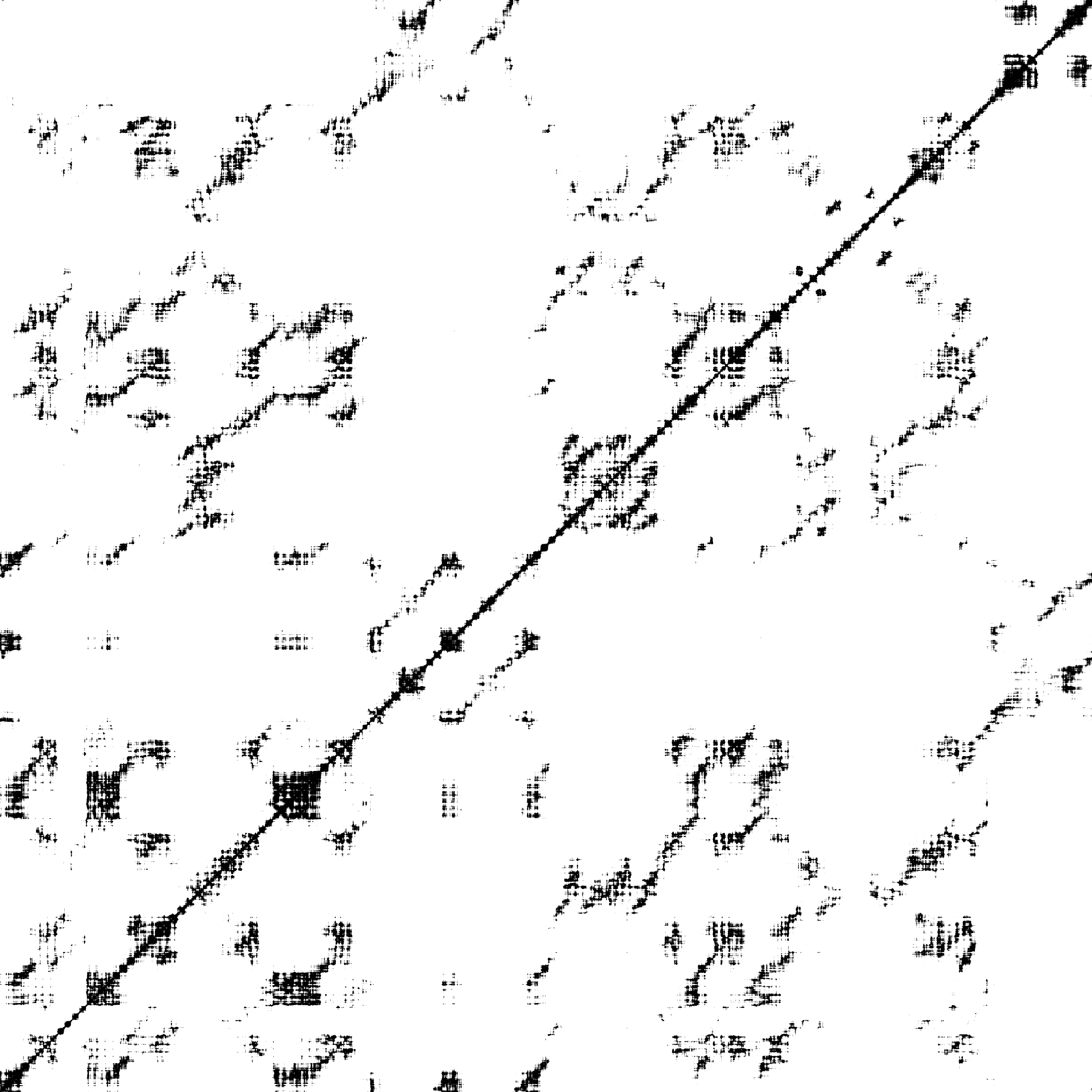
Ratio laminarity / determinism (LAM/DET): 1.014530You can also save the Recurrence Plot.
RPcomputation <- pyrqa$computation$RPComputation$create(settings)
RPresult <- RPcomputation$run()
pyrqa$image_generator$ImageGenerator$save_recurrence_plot(RPresult$recurrence_matrix_reverse,'recurrence_plot_python.png')knitr::include_graphics("images/recurrence_plot_python.png")
Figure 12.1: RP produced by PyRQA