3.1 It’s a line! It’s a plane!

The formula resembles the equation of a line. One could consider the value \(Y_{0}\) a constant like the intercept of a line. The proportion of the value of \(Y\) at time \(i\) by which \(Y\) changes is given by parameter \(a\). This is similar to the slope of a line. However, in a 2D \((X,Y)\) plane there are two ‘spatial’ (metric) dimensions representing the values two variables \(X\) and \(Y\) can take on (see figure), in the case of a time series model, the \(X\)-axis represents the time dimension.

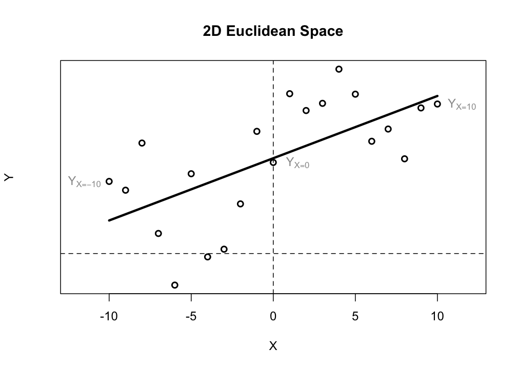
The best fitting straight line through the points in the \((X,Y)\) plane is called a statistical model of the linear relationship between the observed values of \(X\) and \(Y\). It can be obtained by fitting a General Linear Model (GLM) to the data. If \(X\) were to represent repeated measurements the multivariate GLM for repeated measures would have to be fitted to the data. This can be very problematic, because statistical models rely on the assumptions of Ergodic theory:

“… it is the study of the long term average behavior of systems evolving in time.”

The ergodic theorems require a process to be stationary and homogeneous (across time and/or different realisations of the process, i.e. between different individuals).

In other words: If you throw 1 die 100 times in a row, the average of the 100 numbers is the time-average of one of the observables of die-throwing systems. If this system is ergodic, then its time-average is expected to be similar to the average of the numbers that turn up if you throw 100 dice all at the same instance of time. The dice layed out on the table represent a spatial sample, a snapshot frozen in time, of the possible states the system can be in. Taking the average would be the spatial average this observable of die-throwing systems. This ergodic condiciotn is often implicitly assumed in Behavioural Science when studies claim to study change by taking different samples of individuals (snapshots of system states) and comparing if they are the same.

One also needs to assume the independence of measurements within and between individual realisations of the process. These assumptions can be translated to certain conditions that must hold for a (multivariate) statistical model to be valid. Some well known conditions are Compound Symmetry and Sphericity:

The compound symmetry assumption requires that the variances (pooled within-group) and covariances (across subjects) of the different repeated measures are homogeneous (identical). This is a sufficient condition for the univariate F test for repeated measures to be valid (i.e., for the reported F values to actually follow the F distribution). However, it is not a necessary condition. The sphericity assumption is a necessary and sufficient condition for the F test to be valid; it states that the within-subject “model” consists of independent (orthogonal) components. The nature of these assumptions, and the effects of violations are usually not well-described in ANOVA textbooks; [^assumptions]

As you can read in the quoted text above, these conditions must hold in order to be able to identify unique independent components (i.e. the linear predictor \(X\)) as the sources of variation of \(Y\) over time within a subject.

If you choose to use GLM repeated measures to model change over time, you will only be able to infer independent components that are responsible for the time-evolution of \(Y\). As is hinted in the last sentence of the quote, the validity of such inferences is not a common topic of discussion statistics textbooks.