15.1 Recurrence Networks
Recurrence networks are graphs created from a recurrence matrix. This means the nodes (vertices) of the graph represent values observed at specific time points and the connections (edges) between nodes represent a recurrence relation between the values observed at those time points. In a reconstructed or multidimensional (coarse grained) state space, the values represent some measure of distance between the observed states (coordinates in state space).
We can turn the recurrence matrix into an adjacency matrix, e.g. an igraph object in R. This means we can use all the igraph functions to calculate network measures. The main differences between the recurrence matrix as used for (C)RQA and the adjacency matrix is that the latter can represent weighted, as well as directed recurrence networks. The interpretation of the network measures calculated from a recurrence network is somewhat different from when the nodes do not represent time. The ultimate reference for learning about recurrence networks is:
Package casnet has some functions to create recurrence networks, they are similar to the functions used for CRQA:
* rn() is very similar to rp(), it will create a matrix based on embedding parameters, or on a multivariate dataset. One difference is the option to create a weighted and/or directed matrix. This is a matrix in which non-recurring values are set to 0, but the recurring values are not replaced by a 1, the distance value (or recurrence time) is retained and acts as an edge-weight
* rn_plot() will produce similar plots as rp_plot(), with some differences for weighted and directed networks
* rn_measures() produces several common network measures used with recurrence networks.
ESM data
We’ll use the same dataset as in the vignette Dynamic Complexity by Bastiaansen et al. (2019). Load it from the Open Science Framework, or use the internal data.
library(casnet)
library(invctr)
# # Load data from OSF https://osf.io/tcnpd/
# require(osfr)
# manyAnalystsESM <- rio::import(osfr::osf_download(osfr::osf_retrieve_file("tcnpd") , overwrite = TRUE)$local_path)

# Or use the internal data
data(manyAnalystsESM)
A visual inspection of the data reveals some variables can be omitted and cases with missing values need to be imputed or removed. We’ll use the same strategy as explained in the Dynamic Complexity vignette.
library(tidyverse)
library(igraph)

plotTS_multi(manyAnalystsESM, subtitle = "Raw data")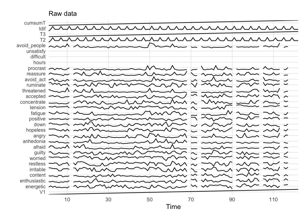
# Use the date information in the dataset to create time series objects
dates   <- format(strptime(manyAnalystsESM$start[!is.na(manyAnalystsESM$start)], "%m/%d/%Y %H:%M"), "%d-%m-%Y\n%H:%M")
weeknum <- as.numeric(format(strptime(manyAnalystsESM$start[!is.na(manyAnalystsESM$start)], "%m/%d/%Y %H:%M"),format = "%V"))

# days       <- format(strptime(dates, "%m/%d/%Y %H:%M"), "%d-%m-%Y")
# time       <- format(strptime(dates, "%m/%d/%Y %H:%M"), "%H:%M")

# Don't use columns 1, 26-28, 30-35
df <- manyAnalystsESM[,-c(1:3, 26:28, 30:35)]

# 1. Remove NA
out.NA <- df[stats::complete.cases(df),]

# 2. Classification And Regression Trees / Random Forests
imp.cart  <- mice::mice(df, method = 'cart', printFlag = FALSE)
out.cart  <- mice::complete(imp.cart)

out.cart$dates <- dates
plotTS_multi(out.cart, subtitle = "Imputed data", timeVec = "dates"%ci%out.cart)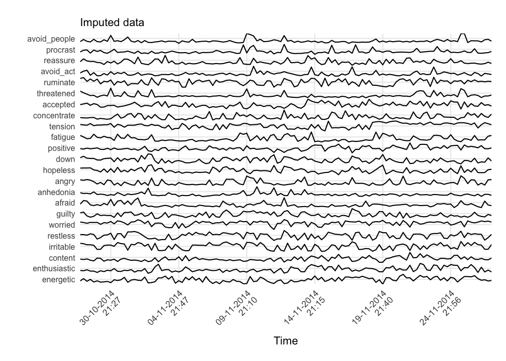
The first step is to create a recurrence matrix and consider it an adjacency matrix. This matrix can be created based on the reconstructed state space using the method of delay embedding, or, on a multidimensional state space in which the dimensions are a (subset) of the multivariate time series.