6.2 Standardised Dispersion Analysis (SDA)

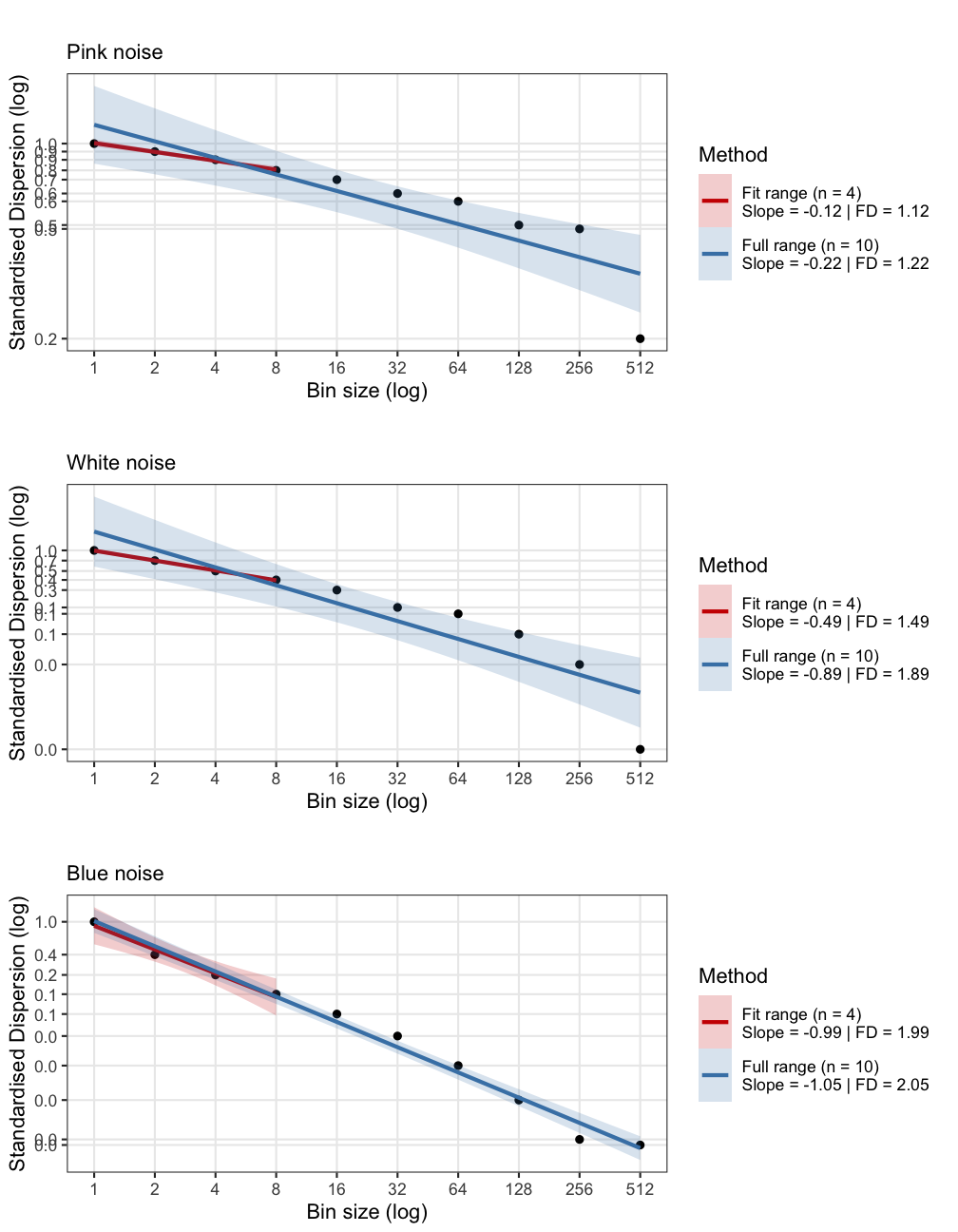
In Standardised Dispersion Analysis, the time series is converted to z0scores (standardised) and the way the average standard deviation (SD) calculated in bins of a particular size scales with the bin size should be an indication of the presence of power-laws. That is, if the bins get larger and the variability decreases, there probably is no scaling relation. If the SD systematically increases either with larger bin sizes, or, in reverse, this means the fluctuations depend on the size of the bins, the size of the measurement stick.

sdaN1 <- fd_sda(ColouredNoise$`-1`, doPlot = FALSE, returnPlot = TRUE, tsName = "Pink noise", noTitle = TRUE)

> 
> 
> (mf)dfa:  Sample rate was set to 1.
> 
> 
> ~~~o~~o~~casnet~~o~~o~~~
> 
>  Standardised Dispersion Analysis 
> 
>  Full range (n = 10)
> Slope = -0.22 | FD = 1.22 
> 
>  Fit range (n = 4)
> Slope = -0.12 | FD = 1.12
> 
> ~~~o~~o~~casnet~~o~~o~~~

sda0  <- fd_sda(ColouredNoise$`0`, doPlot = FALSE, returnPlot = TRUE, tsName = "White noise", noTitle = TRUE)

> 
> 
> (mf)dfa:  Sample rate was set to 1.
> 
> 
> ~~~o~~o~~casnet~~o~~o~~~
> 
>  Standardised Dispersion Analysis 
> 
>  Full range (n = 10)
> Slope = -0.89 | FD = 1.89 
> 
>  Fit range (n = 4)
> Slope = -0.49 | FD = 1.49
> 
> ~~~o~~o~~casnet~~o~~o~~~

sdaP1 <- fd_sda(ColouredNoise$`1`, doPlot = FALSE, returnPlot = TRUE, tsName = "Blue noise", noTitle = TRUE)

> 
> 
> (mf)dfa:  Sample rate was set to 1.
> 
> 
> ~~~o~~o~~casnet~~o~~o~~~
> 
>  Standardised Dispersion Analysis 
> 
>  Full range (n = 10)
> Slope = -1.05 | FD = 2.05 
> 
>  Fit range (n = 4)
> Slope = -0.99 | FD = 1.99
> 
> ~~~o~~o~~casnet~~o~~o~~~

cowplot::plot_grid(sdaN1$plot,sda0$plot,sdaP1$plot,ncol = 1)