5.2 Entropy

Entropy is an important topic, but also often a misunderstood concept. See the Study Materials and Resources of this chapter for some excellent explanations of this quantity. Here we provide an explanation of Entropy based on its meaning in information theory.

Physical Information and Entropy

Classical, algorithmic and quantum information theory explicitly exclude meaningful, or, semantic information as part of their explanatory domain (cf. Desurvire, 2009, p. 38), or, as Shannon lucidly explained:

“The fundamental problem of communication is that of reproducing at one point either exactly or approximately a message selected at another point. Frequently the messages have meaning; that is, they refer to or are correlated according to some system with certain physical or conceptual entities. These semantic aspects of communication are irrelevant to the engineering problem. The significant aspect is that the actual message is one selected from a set of possible messages. The system must be designed to operate for each possible selection, not just the one which will actually be chosen since this is unknown at the time of design.” (Shannon, 1948, p. 379, emphasis in original)

The semantic aspects of a message are irrelevant for reproducing it, if they were relevant for message reproduction, a universal theory of information and communication would not be possible. In order to successfully communicate a message through a channel if semantics were involved, one would have to know particular facts about these correlations with “some system with certain physical or conceptual entities”. What then is information?

In the most general terms, information can be defined as a quantity that resolves uncertainty about the state of an information source, a physical entity that can represent an amount of information. The information-theoretic quantity known as self-information, or information content (\(I\)) quantifies the reduction of uncertainty due to the observation of a particular state of the information source. For example, an information source that can be in 2 states, a fair coin, can represent 2 bits of information (2 things to be uncertain about). Observing 1 of the 2 possible states (‘heads’) resolves uncertainty about the state of the system by an amount of 1 bit of information.

Another important information-theoretic quantity is entropy (\(H\)), which can be interpreted as the expected value of \(I\) over repeated observations of states of the information source. For a fair coin, the 2 possible states are equiprobable, so the expected amount of information represented by the observation either ‘heads’ or ‘tails’ will be 1. Figure 5.4 displays the relation between the information and entropy represented by each state for different configurations of the coin: Biased towards ‘Tails’ (\(Pr(X=Heads)<.5\)); fair (\(Pr(X=Heads)=.5\)); biased towards ‘Heads’ (\(Pr(X=Heads)>.5\)). The dotted lines show the Information represented by the observation of \(X=Heads\) or \(X=Tails\). The entropy is at its maximum \(H = 1\ bit/symbol\) when the system is configured to be fair, In that case the observation of each state would represent the same amount of information (\(I = 1\)). in which case the observation of a particular state does not provide any information about the state that will be observed next, our best guess, is quite literally, to guess.

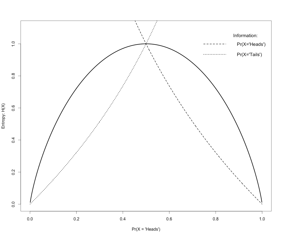
Figure 5.4: Information and Entropy of a coin system.

The maximum entropy state represents maximum unpredictability, in the case of a physical system one would refer to the maximum entropy state as a state of maximum disorder. For now, it is important to note that information is dimensionless in the sense that it does not represent a characteristic scale of observation, but has to be interpreted relative to the scale at which the microscopic states of the system are observed. If a computer scientist and a particle physicist have to estimate the amount of information that is represented by a 1GB memory chip, they will give two different, but correct answers (\(2^{33}\) and \(\approx2^{76}\) bits, respectively). This is due to the scale at which the degrees of freedom of the information source are identified. The computer scientist cares about the on and off states of the transistors on the chip, whereas the particle physicist is more likely interested in the states of billions of individual particles (example taken from Bekenstein, 2003, p. 59).

A user of a 1GB flash drive commonly wants to know whether there is enough free space to copy one or more files onto it. The amount of free space, expressed as a quantity of information, for example, 100MB, refers to the degrees of freedom at the level of the on and off states of the transistors on the chip that are still available to become “correlated according to some system with certain physical or conceptual entities”. We will refer to such degrees of freedom as non-information bearing d.o.f., or, non-informative structure, as opposed to information-bearing d.o.f., or, informative structure. The latter would concern those transistors whose state is temporarily fixed, because they are part of a specific configuration of transistor states that is associated with one or more systems of physical or conceptual entities (i.e. the state encodes for whatever digital content was stored on the drive). The non-informative structure concerns transistors whose state is not fixed, and would be available to become associated to some other system of entities. Another way to describe this situation, is that there has been a (relative) reduction of the total degrees of freedom available to the system, from \(8,589,934,592\) (1GB) to \(838,860,800\) (100MB) on/off states. The informative structure represents systematicity, certainty, order: “order is essentially the arrival of redundancy in a system, a reduction of possibilities’’ (von Foerster, 2003). The non-informative structure represents possibility, uncertainty, disorder.

These quantities of information can be used to distinguish one system state relative to another (e.g. less or more redundancy/possibility, order/disorder, unavailable/available storage space), and this can lead to the emergence of identity (cf. Kak, 1996). However, this is not the same as the emergence of meaning, that is, it the quantity does not account for the emergence of informative structure, which would require knowledge about the system with which the configuration of degrees of freedom became associated. The amount of information represented by an information source does not specify what it codes for, it is meaningless (cf. Küppers, 2013). To ‘make use’ of the meaning encoded in an information source one would need to be able learn the systemic regularities it codes for by observing how the redundancies came about, or, figure out how to translate the configuration into another, known code (an equivalent to the Rosetta stone). Compared to the concept of internal or mental representation, the physical representation of information is much more an indication of a capacity for registering an amount of information (Lloyd, 2006). It refers to a potential for establishing a new order in the configuration of the system by recruiting available degrees of freedom, whereas the mental representations the post-cognitivists seek to dispense with, refer to previously realized order that was somehow trapped, stored, or imprinted into the structure of the system.

Entropy in time series

To estimate the entropy of an observed time series, we need some method for deciding how predictable the series is, what are the redundancies in the series we can exploit in order to know what is going to happen next? We’ll use a measure called Sample Entropy or SampEn, which can be interpreted as measuring the average amount of information that is needed in order to represent all the (patterns) of values observed in the time series. If we need lots of information, this means the time series is unpredictable, random and the SampEn will be high. If we need just a few bits of information, this means the time series is very predictable, deterministic and the SampEn will be low.

More formally: Sample entropy is the negative natural logarithm of the conditional probability that a dataset of length \(N\), having repeated itself within a tolerance \(r\) for \(m\) points, will also repeat itself for \(m+1\) points.

\(P = \frac{distance\ between\ values\ in\ data\ segment\ of\ length\ m+1\ <\ r}{distance\ between\ values\ in\ data\ segment\ of\ length\ m\ <\ r}\)

\(SampEn = −\log P\)

Figure 5.5 can be used to lookup which value of SampEn corresponds to which type of dynamics. As expected, white noise has the highest SampEn, it is the most unpredictable type of noise. The other noises, towards (infra) red and (ultra) violet noise are characterised by increasingly dominant high and low frequency oscillations, which are redundancies, and they make the behaviour of the series predictable.

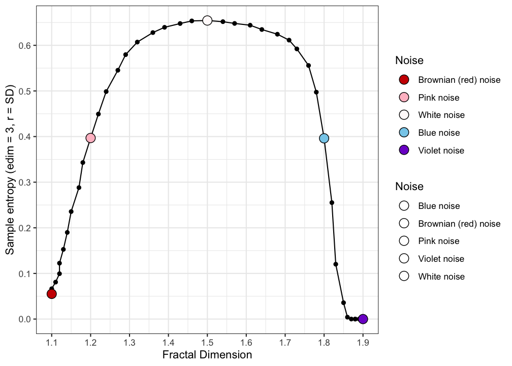
Figure 5.5: Coloured Noise versus Sample Entropy