10.1 Phase Space Reconstruction
A record of all the dimensions that span the phase space of a system will not be available in most cases, so a reconstruction of the attractor and dynamics in phase space will often be conducted. This a common step in many nonlinear time series analyses and can be achieved using the method of delay-embedding (Kantz & Schreiber, 2004; Takens, 1981). 2 Due to Takens’ theorem (1981) a phase space can be reconstructed that is topologically equivalent to the original space, by creating an \(m\)-dimensional time-delay embedding of a single observed dimension of a system: \(\vec{y}_i = (y_i, y_{i+\tau}, \ldots, y_{i+\left(m-1\right)\tau})\), where \(\tau\) is the embedding delay. The idea is to exploit the interaction-dominant dynamics that govern the behavior of complex systems. Due to the coupled dynamics of the 4 dimensions of the simulated system, there is information about the dynamics of \(Y_2\), \(Y_3\) and \(Y_4\) encoded in the dynamics of \(Y_1\). Therefore, any of the dimensions could be used to reconstruct the dynamics of the original phase space. The exact trajectories through phase space will be different, but the dynamical invariants of the original attractor will be retained by the reconstruction and recurrence analyses can be used to quantify (properties of) dynamical invariants. The attractor reconstruction procedure involves two steps, the first is choosing an embedding delay \(\tau\), the second concerns choosing an appropriate number of surrogate dimensions to embed the time series.
10.1.1 Choosing an embedding lag
The choice for the embedding delay is an optimization step and less crucial than choosing a sufficiently large embedding dimension. Takens’ theorem guarantees topological equivalence if \(m\) is twice as large as the fractal dimension of the support (the nonzero elements) of the invariants generated by the dynamics in the original phase space (Zou et al., 2019). In other words, there should be enough nonzero data to make an embedding with enough surrogate dimensions that fully captures the original dynamics. Embedding a time series in a higher dimension than strictly necessary is unproblematic. Intuitively, \(\tau\) should represent a lag of time at which the information about future states of the system as predicted by its history, are at a minimum, for example, the lag at which the autocorrelation function goes to \(0\). However, because time series representing observables of complex systems more often than not violate the stationarity and homogeneity assumptions, a time-delayed mutual information function is commonly used (cf. Fraser & Swinney, 1986). As can be seen in the top panel of Figure 10.3 the mutual information function of dimension \(Y_1\) has local and global minima that could be used as the embedding delay. A delay of 17.5 was used (the median of the first local minima found for the four series) for all reconstructions. By copying the time series starting at \(\tau\) and treating it as the first point of a surrogate dimension, a state vector is created based on a single observed time series. This process is repeated up to \(m\)-dimensions, by copying the series at \(2\tau, 3\tau,\ldots (m-1)\tau\). The question is, how to decide on the number of embedding dimensions required to represent the dynamics of the original attractor?
10.1.2 False Nearest Neighbor analysis
One way to estimate \(m\) is by False Nearest Neighbor (FNN) analysis (Kennel, Brown, & Abarbanel, 1992), which will consider whether points that are close together in an \(m\)-dimensional reconstructed phase space, will still be close together in an \(m+1\) embedding. If this is not the case, these points were ‘false neighbors’ of the points in \(m\) dimensions. The lower panel of Figure 10.3 shows the results of the FNN analysis for the simulated system. We know the correct number of dimensions should be \(m = 4\) and this is indeed the case for \(Y_1\) and the local minimum. With real-world data, one would look at the dotted line, where the percentage of false neighbors drops below 10%. The value obtained by FNN provides an estimate of the minimum number of coupled ODE’s required to model the dynamics of the original phase space trajectory. Based on \(Y_2\) and \(Y_4\) a similar result is found, but \(Y_3\) is an exception, here FNN indicates a much higher embedding dimension. The reason is the lack of support that is required by Takens’ theorem, as can be seen in Figure 10.1, series \(Y3\) contains a lot of zeroes. If this were an observed data set and the aim was to compare analyses based on reconstructions of each of the four series, the largest embedding dimension would be used for all series, for demonstration purposes, we’ll use \(m=4\) for all reconstructions. Note that the lack of support in \(Y_3\) cannot be resolved by simply adding a constant and proceeding with attractor reconstruction. The lack of support is produced by the coupled dynamics, so there are basically two ways in which \(Y_3\) could become a candidate for a successful phase space reconstruction: i) Observe the dynamics for a longer period of time, potentially decreasing the relative frequency of zeros; ii) Change the parameters to change the dynamics of \(Y_3\).
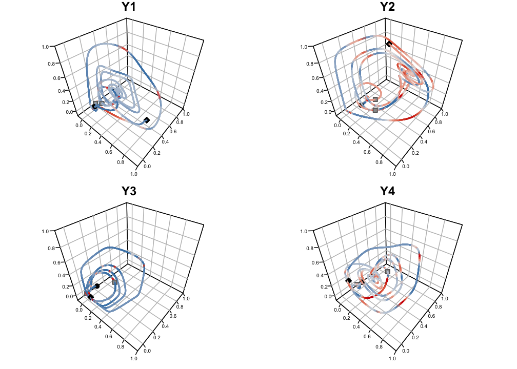
Figure 10.5: The reconstructed phase space based on variable Y1, Y2, Y3 and Y4 respectively. The black diamond indicates t=0; the grey squares at t=700 and t=800 indicate where the coupling strength is increased; the black circle is at t=949.
The Figure displays reconstructed attractors based on each of the 4 dimensions. The topological equivalence may not be immediately apparent, but considering that for each reconstruction just 1 of the original dimensions was used it is quite remarkable we end up with a trajectory that appears to orbit around a specific region. According to the rules of topology, there exists a continuous deformation for each of these trajectories that will recover the exact same shape as the original attractor. The topological equivalence is visible in the unthresholded distance matrices displayed in Figure 10.6. Here, the transition towards the stable state that persists for some time is clearly visible, as well as several other transitions to states that recur for a shorter duration of time.
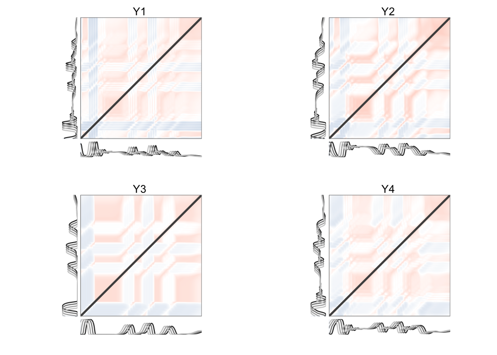
Figure 10.6: Distance matrix of the reconstructed phase spaces based on Y1, Y2, Y3, and Y4, respectively.
The next step is to either turn the thresholded recurrence matrix into a Recurrence Plot (RP, Eckmann, Kamphorst, & Ruelle, 1987; Marwan et al., 2007; Webber Jr & Zbilut, 1994), or into a Recurrence Network (RN, Zou et al., 2019).
Note that phase space reconstruction is not strictly necessary for recurrence quantification analysis and recurrence network analysis. The analyses presented in this paper can also be conducted on the non-embedded ‘raw’ time series, however, here we assume the embedded series to be more informative.↩︎