B.4 Using ggplot2 | The Complex Systems Approach to Behavioural Science

B.4 Using `ggplot2`

Becoming proficient at ggplot2 can take some time, but it does pay off. One of the problems with plotting time series data is that ggplot2 wants tidy data in long format. Tidy data is:

Tidy data is a standard way of mapping the meaning of a dataset to its structure. A dataset is messy or tidy depending on how rows, columns and tables are matched up with observations, variables and types. In tidy data: 1. Each variable forms a column. 2. Each observation forms a row. 3. Each type of observational unit forms a table.

—Wickham et al. (2014)

So if we have a set of time series as in the previous examples, we need to change it to long format.

library(tidyverse)

# A wide data frame
df.wide <- data.frame(rnormY        = Y,
                      cumsumY       = cumsum(Y), 
                      centercumsumY = cumsum(ts_center(Y)),
                      time          = seq_along(Y)
                      )

glimpse(df.wide)

> Rows: 100
> Columns: 4
> $ rnormY        <dbl> 0.78482166, 0.19776074, 1.07957851, 1.52605836, 0.400260…
> $ cumsumY       <dbl> 0.7848217, 0.9825824, 2.0621609, 3.5882193, 3.9884794, 4…
> $ centercumsumY <dbl> 0.6249966, 0.6629322, 1.5826857, 2.9489189, 3.1893540, 3…
> $ time          <int> 1, 2, 3, 4, 5, 6, 7, 8, 9, 10, 11, 12, 13, 14, 15, 16, 1…

# Create a long dataframe using gather()
df.long <- df.wide %>% 
  gather(key=TimeSeries,value=Y,-"time")

glimpse(df.long)

> Rows: 300
> Columns: 3
> $ time       <int> 1, 2, 3, 4, 5, 6, 7, 8, 9, 10, 11, 12, 13, 14, 15, 16, 17, …
> $ TimeSeries <chr> "rnormY", "rnormY", "rnormY", "rnormY", "rnormY", "rnormY",…
> $ Y          <dbl> 0.78482166, 0.19776074, 1.07957851, 1.52605836, 0.40026016,…

# 1 plot
ggplot(df.long, aes(x=time, y=Y, colour=TimeSeries)) +
  geom_line() +
  theme_bw()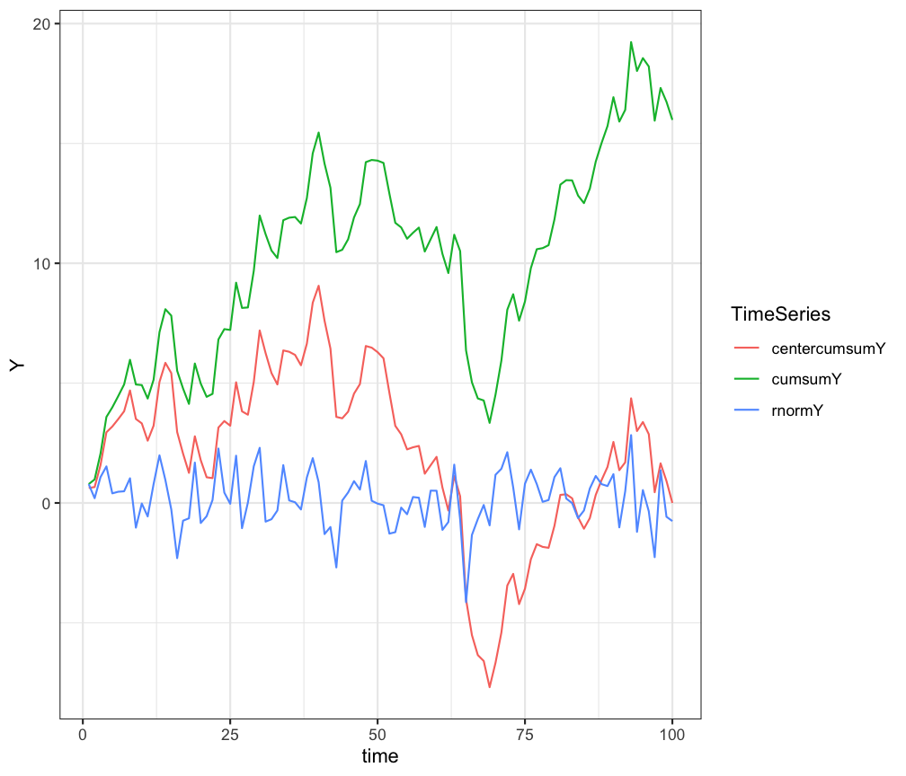

# using facets
ggplot(df.long, aes(x=time,y=Y)) +
  geom_line() + 
  facet_wrap(~TimeSeries) +
  theme_bw()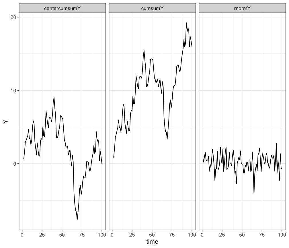

# using facets
ggplot(df.long, aes(x=time,y=Y)) +
  geom_line() + 
  facet_grid(TimeSeries~.) +
  theme_bw()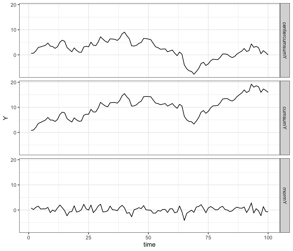

To create a return plot you can use geom_path() instead of geom_line() and make the area square using coord_equal().

# Add a lagged variable
df.long <- df.long %>%
  group_by(TimeSeries) %>%
  mutate(Ylag = dplyr::lag(Y))

# Use geom-path()
ggplot(df.long, aes(x=Y,y=Ylag,group=TimeSeries)) +
  geom_path() + 
  facet_grid(.~TimeSeries) +
  theme_bw() +
  labs(title = "Equal coordinates", x="Yt",y="Yt+1") +
  coord_equal()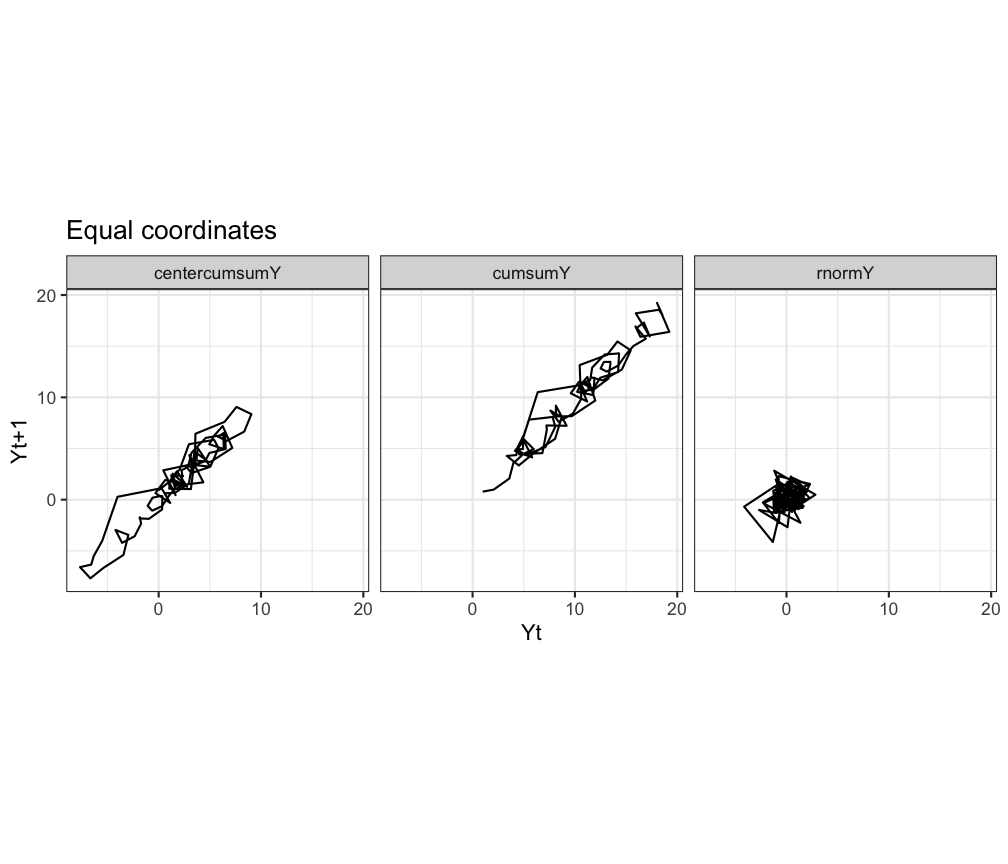

# You could also have free axes
ggplot(df.long, aes(x=Y,y=Ylag,group=TimeSeries)) +
  geom_path() + 
  facet_grid(.~TimeSeries, scales = 'free') +
  labs(title="Free axes", x="Yt",y="Yt+1") +
  theme_bw()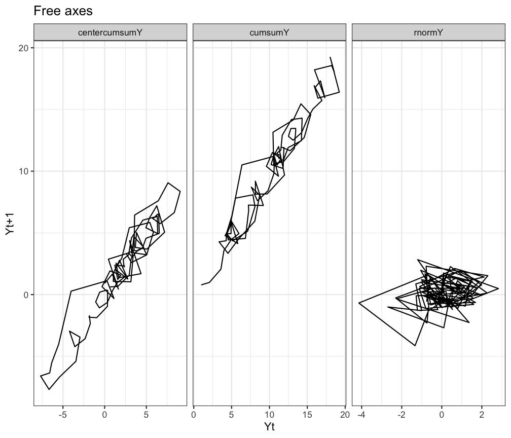

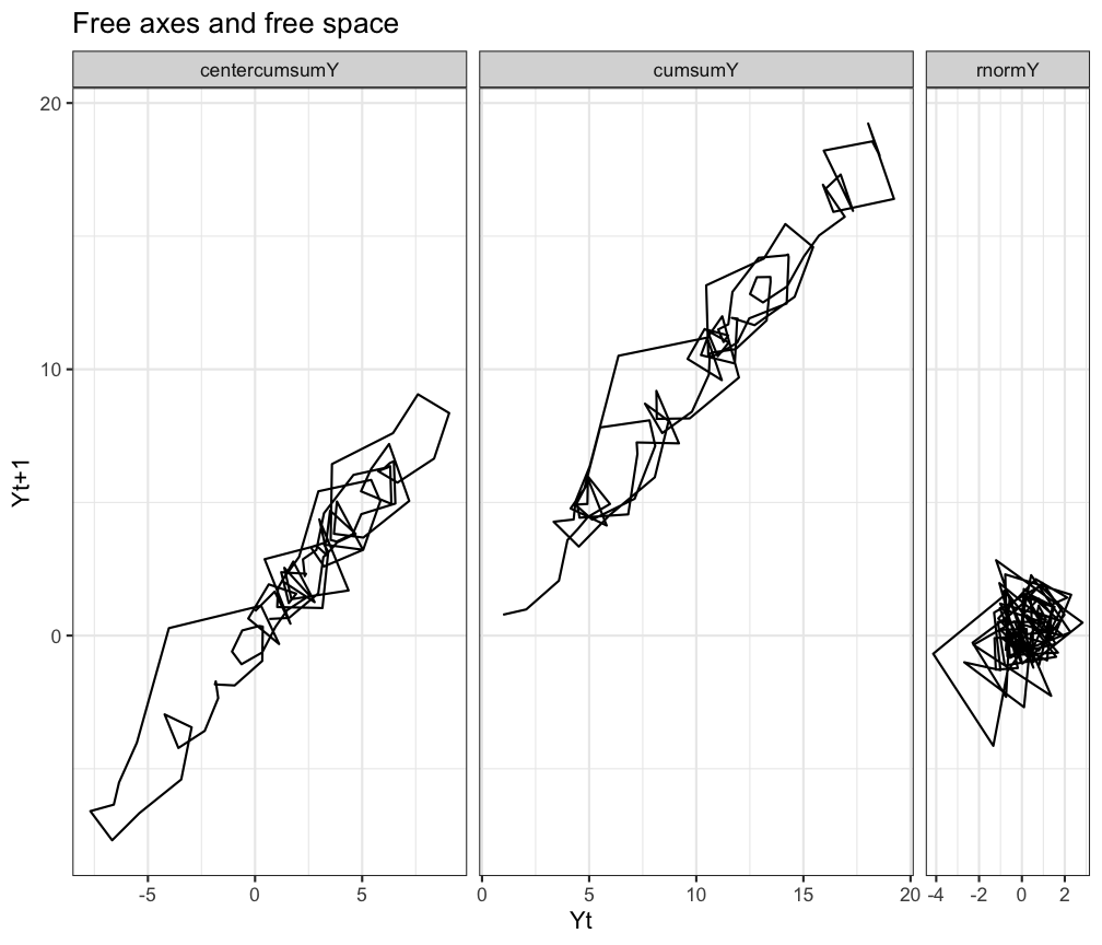
# Or free axes and a free space
ggplot(df.long, aes(x=Y,y=Ylag,group=TimeSeries)) +
  geom_path() + 
  facet_grid(.~TimeSeries, scales = 'free', space = 'free') +
  labs(title="Free axes and free space", x="Yt",y="Yt+1") +
  theme_bw()