B.2 Plotting multiple time series in one figure

Plot multiple time series in frames with plot.ts() in package::stats. This function takes a matrix as input, here we use cbind( ... ).

# stats::plot.ts  
plot(cbind(Y,
           cumsum(Y), 
           cumsum(ts_center(Y))
           ), 
     yax.flip = TRUE, col = "blue", frame.plot = TRUE, 
     main = expression(paste("Random Numbers: ",N(0,sigma))), xlab = "time (a.u.)")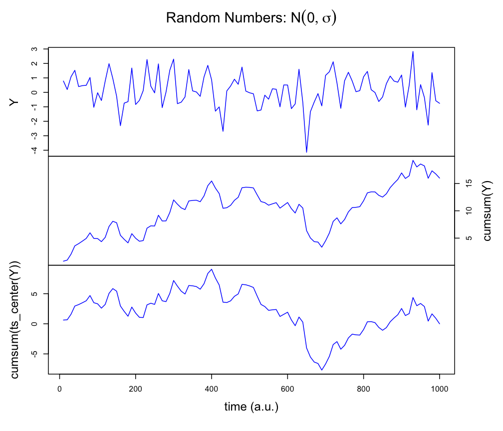

Plot multiple time series in one graph with ts.plot() in package::graphics. This function can handle multiple ts objects as arguments.

# graphics::ts.plot
ts.plot(Y,
        cumsum(Y), 
        cumsum(ts_center(Y)),
        gpars = list(xlab = "time (a.u.)",
                     ylab = expression(Y(t)),
                     main = expression(paste("Random Numbers: ",N(0,sigma))),
                     lwd = rep(2,3),
                     lty = c(1:3),
                     col = c("darkred","darkblue","darkgreen")
                     )
        )
legend(0, 18, c("Y","cumsum(Y)", "cumsum(ts_center(Y))"), lwd = rep(2,3), lty = c(1:3), col = c("darkred","darkblue","darkgreen"), merge = TRUE, cex=.9)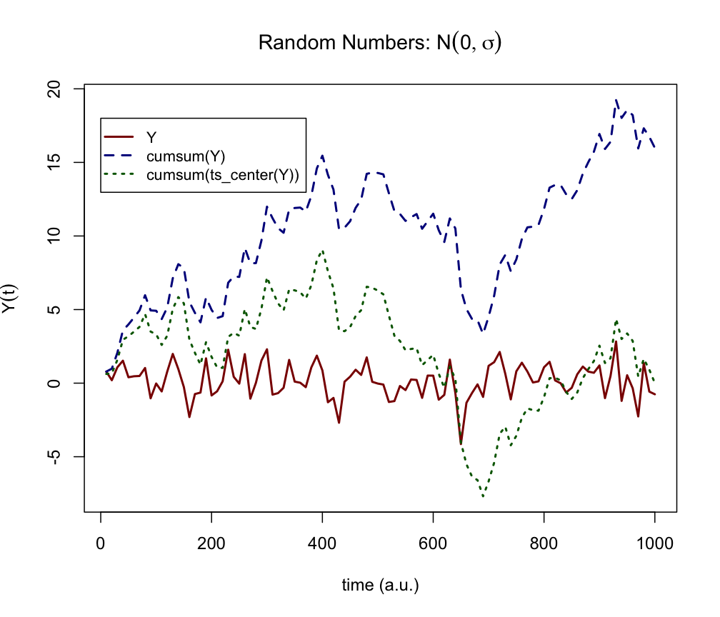

Use xyplot() in package::lattice to create a plot with panels. The easiest way to do this is to create a dataset in so-called “long” format. This means the variable to plot is in 1 column and other variables indicate different levels, or conditions under which the variable was observed or simulated.

Function ldply() is used to generate \(Y\) for three different settings of \(r\). The values of \(r\) are passed as a list and after a function is applied the result is returned as a dataframe.

require(plyr)          # Needed for function ldply()

# Create a long format dataframe for various values for `r`
data <- cbind.data.frame(Y     = c(as.numeric(Y), cumsum(Y), cumsum(ts_center(Y))),
                         time  = c(time(Y), time(Y), time(Y)),
                         label = factor(c(rep("Y",length(Y)),  rep("cumsum(Y)",length(Y)), rep("cumsum(ts_center(Y))",length(Y))))
                         )
# Plot using the formula interface
xyplot(Y ~ time | label, data = data, type = "l", main = expression(paste("Random Numbers: ",N(0,sigma))))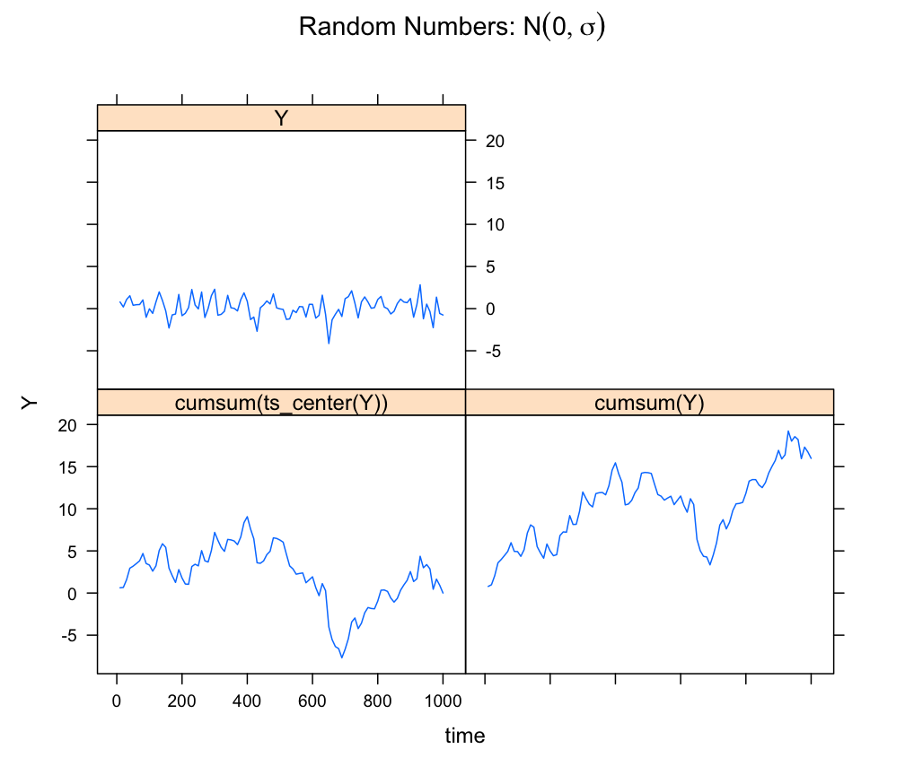

Or, if you have very may time series, you can use the function PLOT() in casnet.

# Create a data frame with time series
# Generate some coloured noise
N <- 512
noises <- seq(-2,2,by=.2)
y <- data.frame(matrix(rep(NA,length(noises)*N), ncol=length(noises)))

for(c in seq_along(noises)){y[,c] <- noise_powerlaw(N=N, alpha = noises[c])}
colnames(y) <- paste0(noises)

plotTS_multi(y)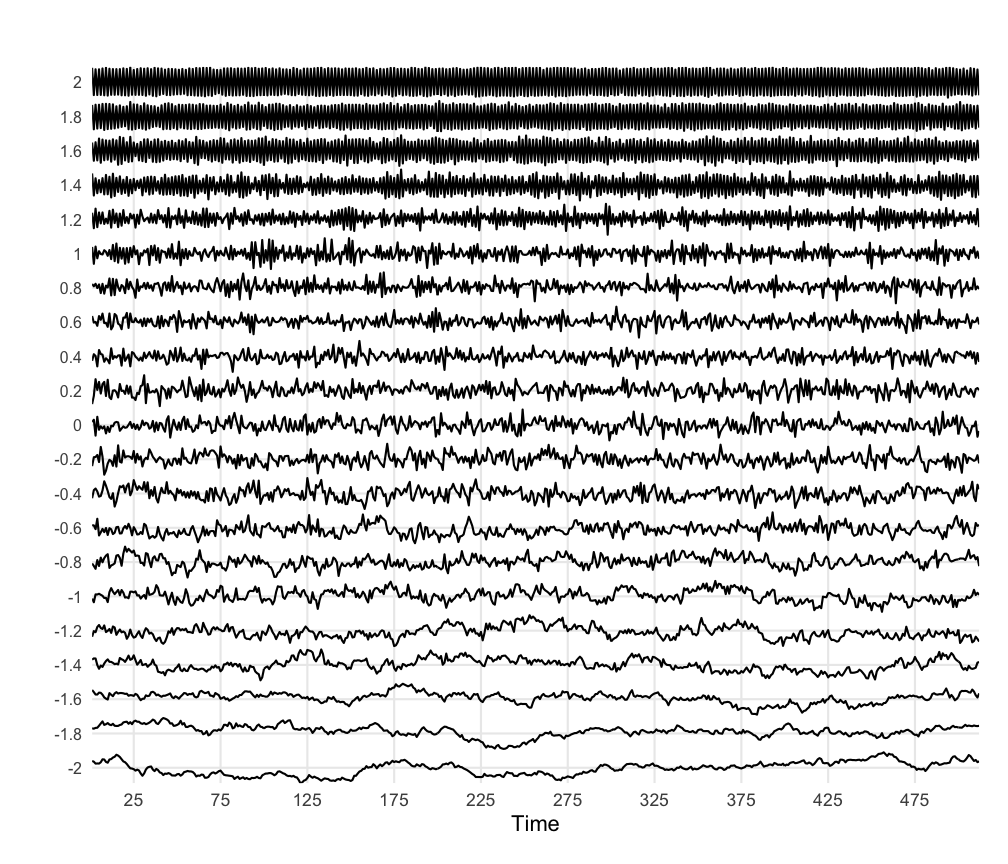

Note that the y-axis is rescaled for each series and does not reflect magnitude differences between the series.