B Working with time series in R

There are many ways to handle time series in R, this appendix provides some examples and suggest some best practices, based on the function ts(), which creates a time series object.

A time series object is expected to have a time-dimension on the x-axis. This is very convenient, because R will generate the time axis for you by looking at the time series properties attribute of the object. Even though we are not working with measurement outcomes, consider a value at a time-index in a time series object a sample:

Start - The value of time at the first sample in the series (e.g., \(0\), or \(1905\))
End - The value of time at the last sample in the series (e.g., \(100\), or \(2005\))
Frequency - The amount of time that passed between two samples, or, the sample rate (e.g., \(0.5\), or \(10\))

Examples of using the time series object.

set.seed(2718282)
# Get a timeseries of 100 random numbers 
Y <- ts(rnorm(100))
# plot.ts
plot(Y)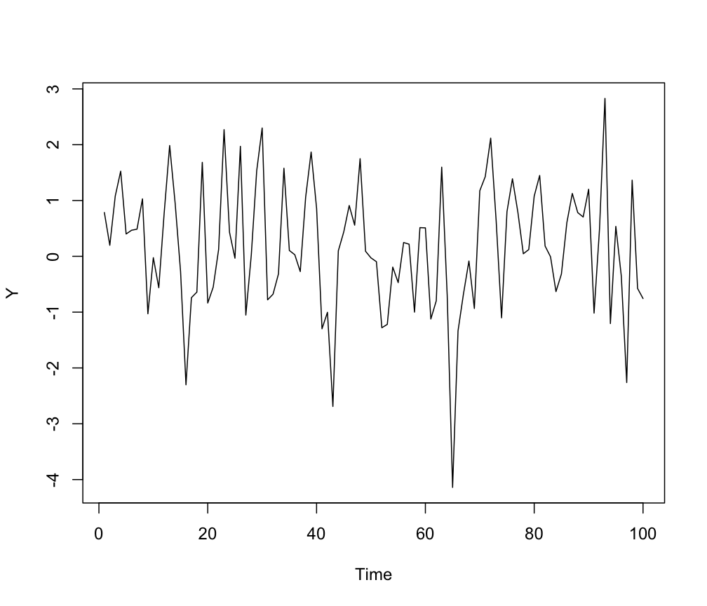

# Get sample rate info
tsp(Y)

> [1]   1 100   1

# Extract the time vector
time(Y)

> Time Series:
> Start = 1 
> End = 100 
> Frequency = 1 
>   [1]   1   2   3   4   5   6   7   8   9  10  11  12  13  14  15  16  17  18
>  [19]  19  20  21  22  23  24  25  26  27  28  29  30  31  32  33  34  35  36
>  [37]  37  38  39  40  41  42  43  44  45  46  47  48  49  50  51  52  53  54
>  [55]  55  56  57  58  59  60  61  62  63  64  65  66  67  68  69  70  71  72
>  [73]  73  74  75  76  77  78  79  80  81  82  83  84  85  86  87  88  89  90
>  [91]  91  92  93  94  95  96  97  98  99 100

For now, these values are in principle all arbitrary units (a.u.). These settings only make sense if they represent the parameters of an actual measurement procedure.

It is easy to adjust the time vector, by assigning new values using tsp() (values have to be possible given the time series length). For example, suppose the sampling frequency was \(0.1\) instead of \(1\) and the Start time was \(10\) and End time was \(1000\).

# Assign new values
(tsp(Y) <- c(10, 1000, .1))

> [1] 1e+01 1e+03 1e-01

# Time axis is automatically adjusted 
time(Y)

> Time Series:
> Start = 10 
> End = 1000 
> Frequency = 0.1 
>   [1]   10   20   30   40   50   60   70   80   90  100  110  120  130  140  150
>  [16]  160  170  180  190  200  210  220  230  240  250  260  270  280  290  300
>  [31]  310  320  330  340  350  360  370  380  390  400  410  420  430  440  450
>  [46]  460  470  480  490  500  510  520  530  540  550  560  570  580  590  600
>  [61]  610  620  630  640  650  660  670  680  690  700  710  720  730  740  750
>  [76]  760  770  780  790  800  810  820  830  840  850  860  870  880  890  900
>  [91]  910  920  930  940  950  960  970  980  990 1000