4.2 Correlation Functions
Correlation functions are intuitive tools for quantifying the temporal structure in a time series. As you know, the correlation measure can only quantify linear regularities between variables, which is why we discuss them here as basic tools for time series analysis. So what are the variables? In the simplest case, the variables between which we calculate a correlation are between a data point at time t and a data point that is separated in time by some lag, for example, if you would calculate the correlation in a lag-1 return plot, you would have calculated the 1st value of the correlation function (actually, it is 2nd value, the 1st value is the correlation of time series with itself, the lag-0 correlation, which is of course \(r = 1\)).
Suppose we have a time series \(Y_i = {1,2,3,4,5,6,5,4,3,2,1}\),
Y <- c(1,2,3,4,5,6,5,4,3,2,1)
plot(ts(Y),type="b")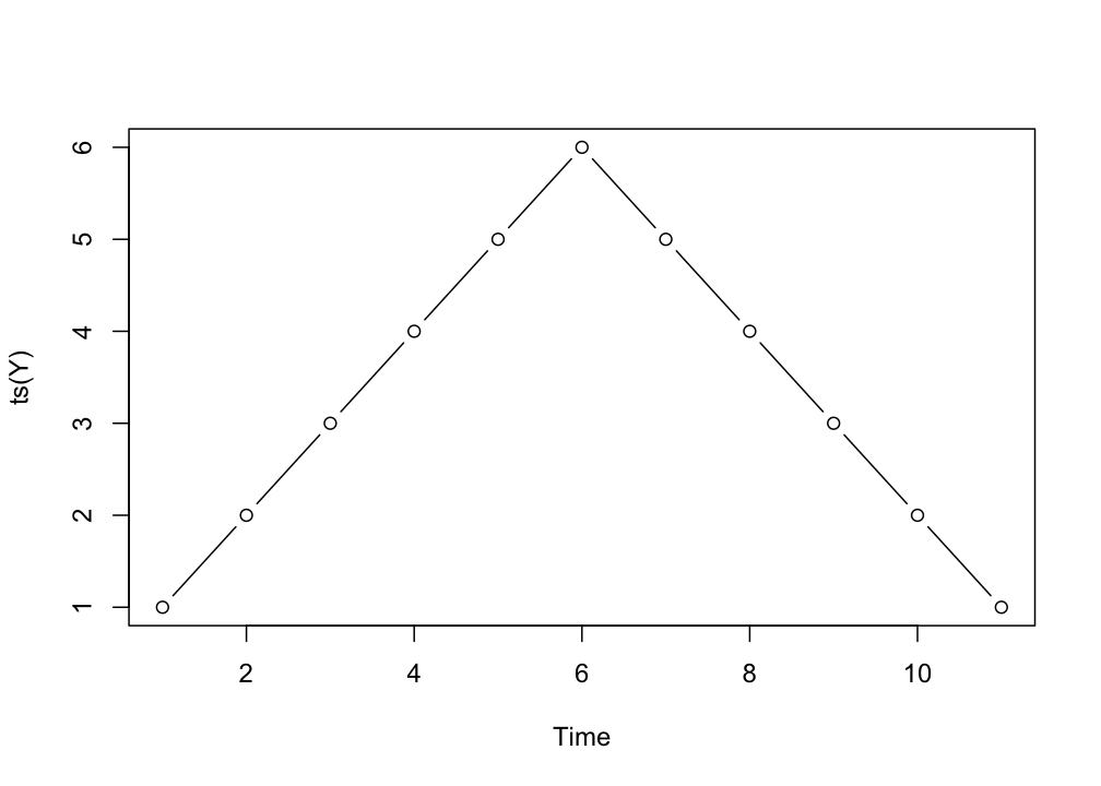
We can create the pairs of lagged values, here we’ll study lags from 0 to 4:
| Y | lag0 | lag1 | lag2 | lag3 | lag4 |
|---|---|---|---|---|---|
| 1 | 1 | 2 | 3 | 4 | 5 |
| 2 | 2 | 3 | 4 | 5 | 6 |
| 3 | 3 | 4 | 5 | 6 | 5 |
| 4 | 4 | 5 | 6 | 5 | 4 |
| 5 | 5 | 6 | 5 | 4 | 3 |
| 6 | 6 | 5 | 4 | 3 | 2 |
| 5 | 5 | 4 | 3 | 2 | 1 |
| 4 | 4 | 3 | 2 | 1 | NA |
| 3 | 3 | 2 | 1 | NA | NA |
| 2 | 2 | 1 | NA | NA | NA |
| 1 | 1 | NA | NA | NA | NA |
Now we can simply calculate the correlation for each pair of Y with a lagged version of Y. This is the auto-correlation, because we are basically comparing Y with itself, just after some lag of time has passed.
(rlag0 <- cor(Y,Y))
> [1] 1
(rlag1 <- cor(Y[1:10],Y[2:11]))
> [1] 0.7777778
(rlag2 <- cor(Y[1:9],Y[3:11]))
> [1] 0.2
(rlag3 <- cor(Y[1:8],Y[4:11]))
> [1] -0.4358974
(rlag4 <- cor(Y[1:7],Y[5:11]))
> [1] -0.8529412
We can plot these correlations to create the so-called autocorrelation function or ACF.
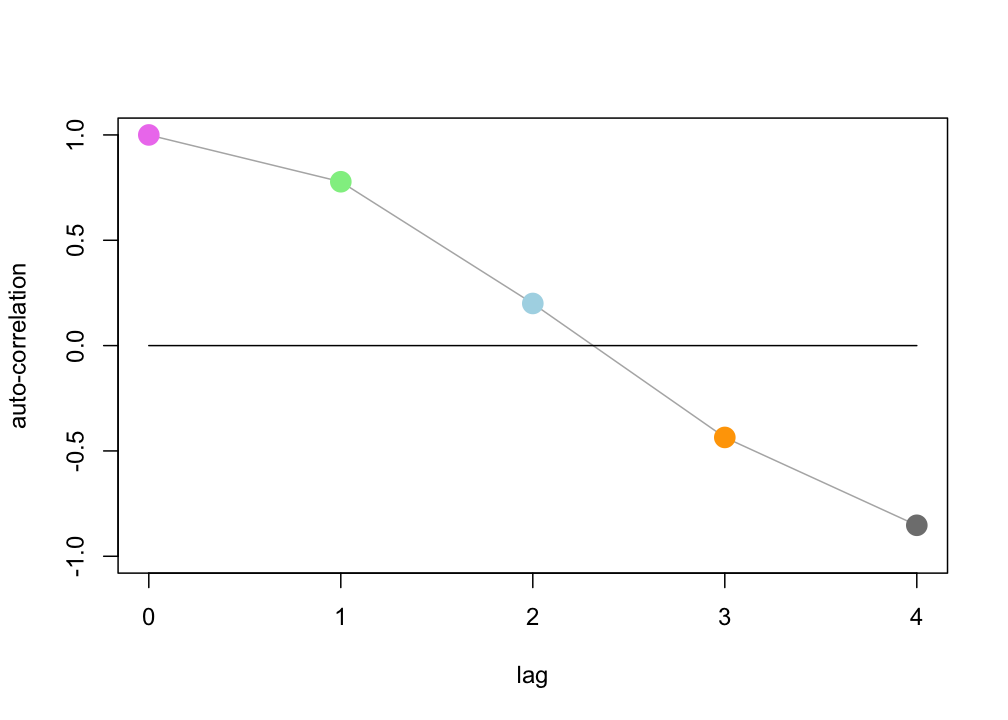
The ACF shows a pattern indicating values separated by a step of 1 are positively correlated (of course, at a lag of 0 the correlation is 1). At lag 4 the correlation is negative, if you look at the plot of the time series you can see that for many time steps the values will be on opposite sides of the peak.
We can also decide whether the correlations deviate significantly from 0. If they do, this can be an indication of ‘memory’, or interdependence: There could be patterns in the data that are recurring with a particular frequency.
In Figure 4.2 the ACF and the partial ACF of a sine wave are shown (using function plotRED_acf()). The partial auto correlation function, ‘partials out’ the correlation that is known from the previous lag and displays the unique correlation that exists between data points seperated by the lags.
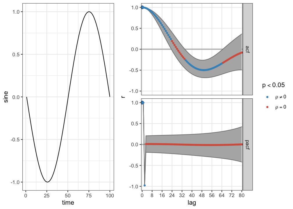
Figure 4.2: (P)ACF of a sine wave