Chapter 10 Continuous Data

Recurrence analyses of continuous data are also based on a recurrence matrix which represents recurring values. In terms of (complex) dynamical systems, recurring values represent states of the system that are re-visited at least once during the time it was observed. There are several different ways to construct a recurrence matrix from one or more time series, in this vignette the recurrence matrix based on phase space reconstruction will be discussed (cf. Marwan, Carmen Romano, Thiel, & Kurths, 2007) as well as the so-called multidimensional recurrence matrix (Wallot, Roepstorff, & Mønster, 2016).

An important concept in recurrence-based time series analyses of continuous data is the Phase (or State) Space and its reconstruction. The state space is spanned by the dimensions of a system and each coordinate in the space represents a potential state of the system (the degrees of freedom available to the system). A sequence of successive states is referred to as a trajectory, or, a path through phase space. If such a trajectory is re-visited by the system, it will be a relatively stable state, or, orbit of the system.

In order to explain the steps involved in reconstructing the phase space from a (multivariate) time series, consider the following system of \(N=4\) coupled competitive Lotka-Volterra equations previously studied by Vano et al. (2006):

\[\begin{equation} \frac{dY_{i}}{dt} = r_iY_i\left(1-\frac{\sum_{j=1}^{N}\alpha_{ij}Y_j}{K_i}\right),\ \ \ i=1,\ldots,N\end{equation}\]

with \(K_i\) the carrying capacity set to a value of \(10\) for all \(Y_i\), and \(r_i\) a vector of growth rates and \(\alpha_{ij}\) a matrix of coupling parameters:

\[\begin{equation} Y_{i}(t=0) = \begin{bmatrix}8\\2\\2\\2\end{bmatrix},\ \ K = \begin{bmatrix}10\\10\\10\\10\end{bmatrix},\ \ r = \begin{bmatrix}1\\0.72\\1.53\\1.27\end{bmatrix},\ \text{and}\ \ \alpha = \begin{bmatrix} 1 &1.09 &1.52 &0\\ 0 &1 &0.44 &1.36\\ 2.33 &0 &1 &0.47\\ 1.21 &0.51 &0.35 &1\end{bmatrix}. \tag{10.1} \end{equation}\]

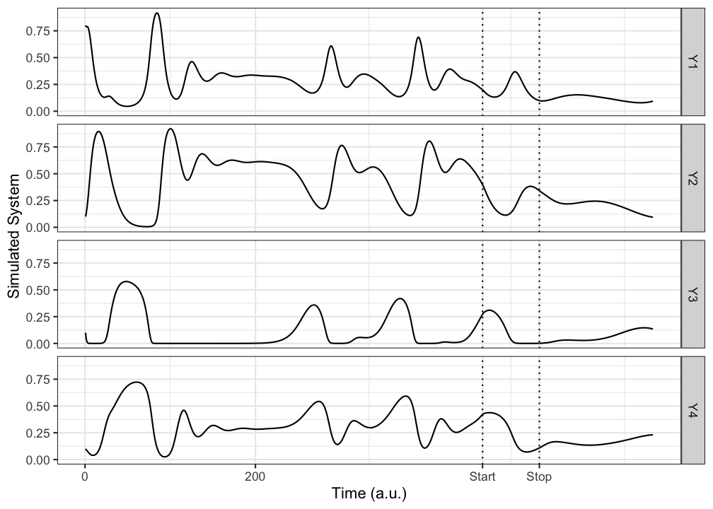
Figure 10.1: Time series representing the dimensions of the 4D system.

The parameters in \(r\) and \(\alpha\) are taken from Vano et al. (2006), who describe the dynamics of the resulting attractor as chaotic (bounded, quasi-periodic, sensitive dependence on initial conditions) and found several quantities to display power-law scaling, which is associated with self-organized criticality of multi-stable complex systems (Bak, Tang, & Wiesenfeld, 1987; Vano et al., 2006). Figure 10.1 shows \(1,000\) iterations of the system (using the 4th order Runge-Kutta method). At \(t=\) 700 the coupling strengths in \(A\) are gradually increased by 0.01 at each iteration untill \(t=\) 800. This means the dynamics of all dimensions become more strongly coupled. These time series could represent a single participant taking part in a study in which bi-daily ratings on a visual analog scale were collected. The dynamics are characterized by initial transient behaviour which settles into a stable, fixed point state, after the coupling strength is changed, a more complex state emerges as a (quasi-)periodic orbit (a trajectory that revisits the same region of phase space, but is not exactly the same as previous visits).

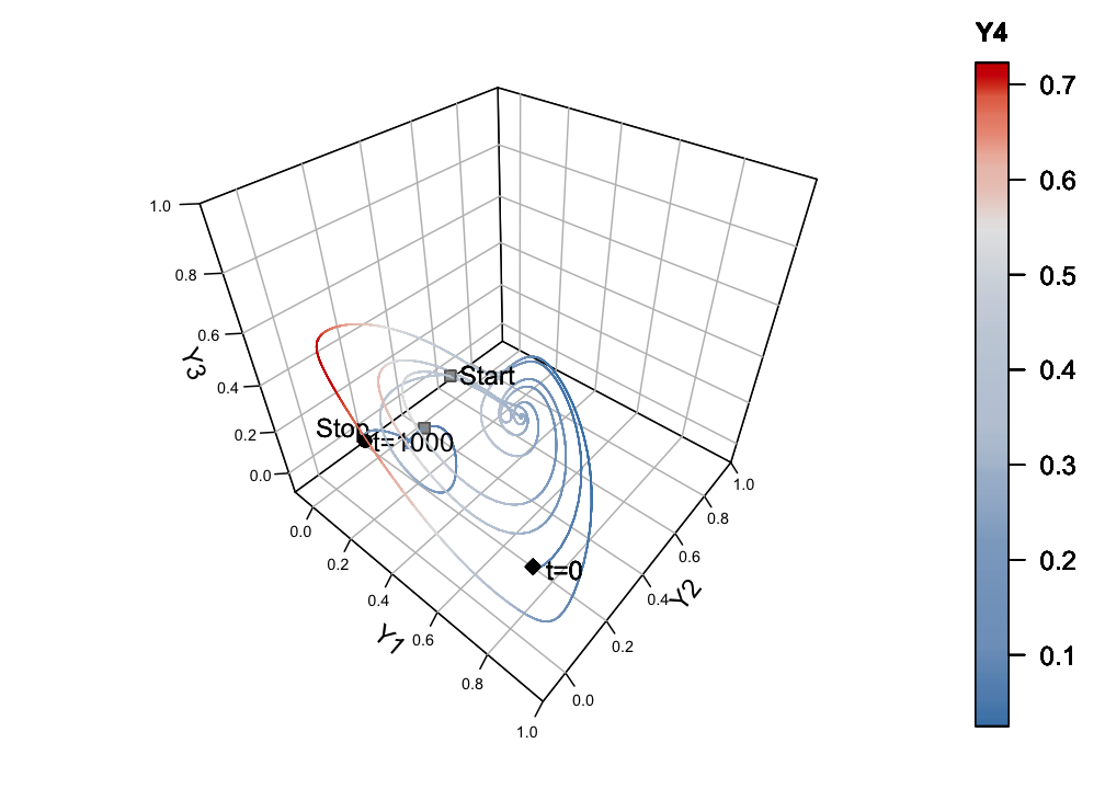
Figure 10.2: The 4D state space of the simulated system. The grey squares mark t=700 and t=800 at which the coupling strengths between the 4 dimensions are gradually increased by 0.01 each iteration.

A (multivariate) time series can be interpreted as a finite representation of the trajectory or state-evolution of a stochastic or deterministic dynamic system: \({y_i}_{i=1}^{N}\), with \(y_i = y(t_i)\) (cf. Zou, Donner, Marwan, Donges, & Kurths, 2019). Figure 10.2 is a 3D representation of the 4D phase space of the system, with the values of dimension \(Y_4\) represented by a colour gradient.

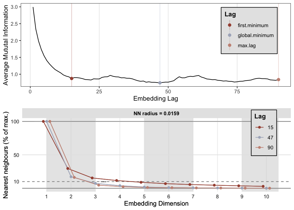
Figure 10.3: Embedding parameters for attractor reconstruction: The upper panel shows the time-delayed mutual information function with 3 embedding delays, 2 minima and the maximum possible lag for 10 surrogate dimensions given the length of the time series. The bottom panel shows the results of the false nearest neighbor analysis for each of the 3 delays. This plot is the ouput of function est_parameters() from package casnet.

The recurrence matrix \(\mathbf{R}_{i,j}\) is defined as: \[\begin{equation} \mathbf{R}_{i,j}(\varepsilon)=\Theta\left(\varepsilon-\|\vec{y}_i-\vec{y}_j\|\right),\ \ \ i,j = 1,\ldots, N \end{equation}\] where \(\|\ \cdot\ \|\) is a distance norm (e.g. Euclidean, Chebyshev, Manhattan), \(\varepsilon\) is a threshold value which determines at which distance value a state should be considered to recur, and \(\Theta\) is the Heaviside function, which returns \(1\) if a distance value falls below \(\varepsilon\) and \(0\) otherwise. Figure 10.4 displays the unthresholded distance matrix based on the Maximum norm (Chebyshev distance). The distances of each state coordinate (a 4-tuple represented by the values of \(y_i\) at each time point) to every other state coordinate are represented by different a colours. The matrix is symmetric around the diagonal, the line of incidence, which is excluded from calculation of recurrence measures. The colour-bar displays several distance values on the right side, which, should they be chosen as the threshold value \(\varepsilon\), would result in the Recurrence Rate (proportion of recurrent points in \(\mathbf{R}_{i,j}\)) displayed on the left.

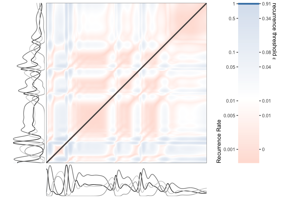
Figure 10.4: Distance matrix of the simulated 4D phase space.