3.3 Implementing iterative functions

Coding change processes (difference equations) in Matlab and R is always easier than using a spreadsheet. One obvious way to do it is to use a counter variable representing the iterations of time in a for ... next loop (see tutorials). The iterations should run over a vector (which is the same concept as a row or a column in a spreadsheet: An indexed array of numbers or characters). The first entry should be the starting value, so the vector index \(1\) represents \(Y_0\).

The loop can be implemented a number of ways, for example as a function which can be called from a script or the command or console window. In R working with functions is easy, and very much recommended (see tutorials), because it will speed up calculations considerably, and it will reduce the amount of code you need to write. You need to gain some experience with coding in R before you’ll get it right. In order to get it lean and clean (and possibly even mean as well) you’ll need a lot of experience with coding in R,therefore, we will (eventually) provide you the functions you’ll need to complete the assignments in the Answers section of the assignments. If you get stuck, look at the answers. If you need to do something that reminds you of an assignment, figure out how to modify the answers to suit your specific needs.

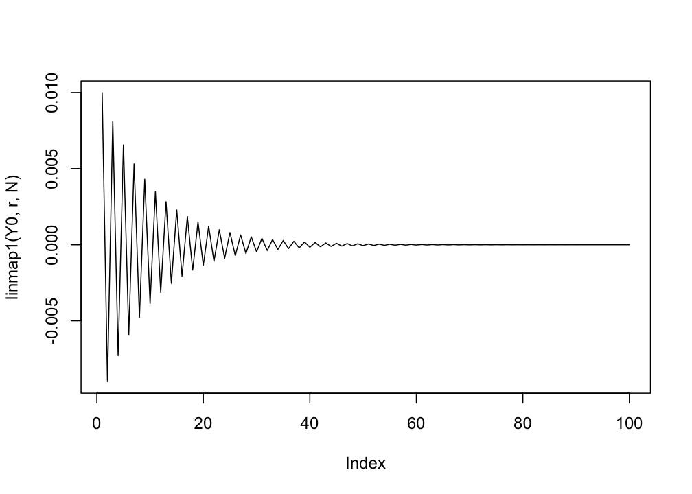
We’ll use the linear map \(Y_{i+1} = r*Y_i\) as an example and show three different ways to implement iterative processes:

The for... loop
The -ply family of functions
User defined function() with arguments

# for loop
N  <- 100
r  <- -.9
Y0 <- 0.01
Y  <- c(Y0,rep(NA,N-1))

for(i in 1:(N-1)){
  Y[i+1] <- r*Y[i]
}
plot(Y,type = "l")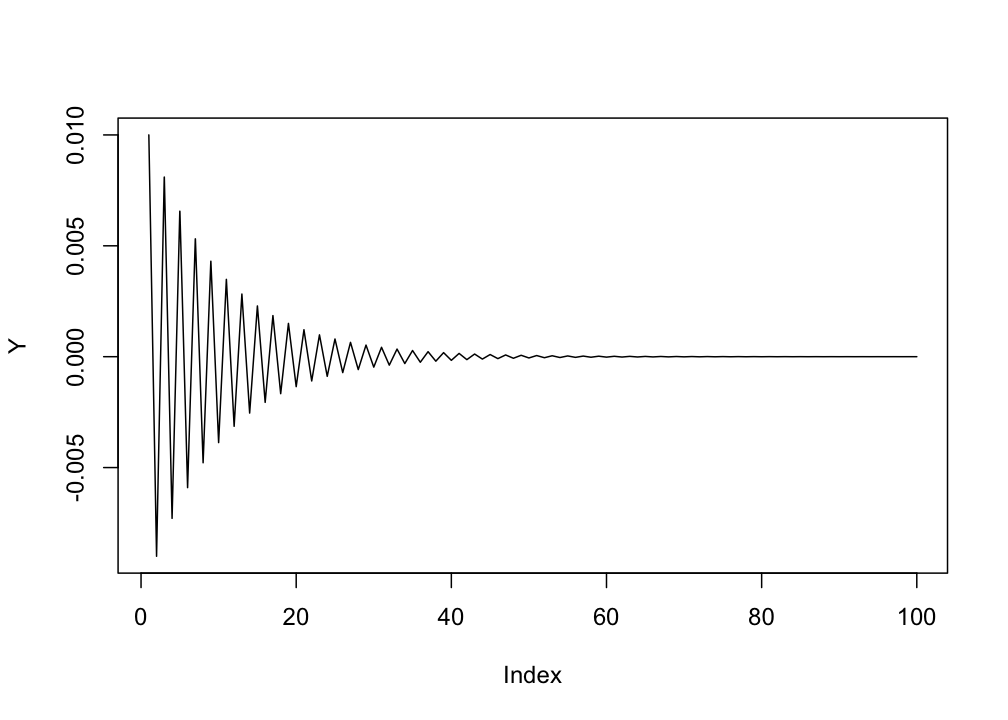

# -ply family: sapply
Yout <- sapply(seq_along(Y),function(t) r*Y[t])
plot(Yout,type = "l")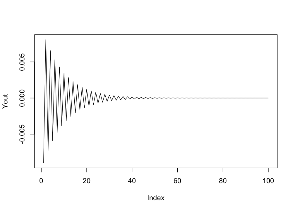

# function with for loop
linmap1 <- function(Y0,r,N){
  Y  <- c(Y0,rep(NA,N-1))
  for(i in 1:(N-1)){
    Y[i+1] <- r*Y[i]
  }
  return(Y)
}
plot(linmap1(Y0,r,N),type = "l")