Reconstructed State Space

Below is an example of how to create a recurrence network based on a reconstructed state space. We’ll examine the variables restless and procrast.

#----------------------
# Adjacency matrix 
#----------------------
library(casnet)

p1 <- est_parameters(y = out.cart$restless)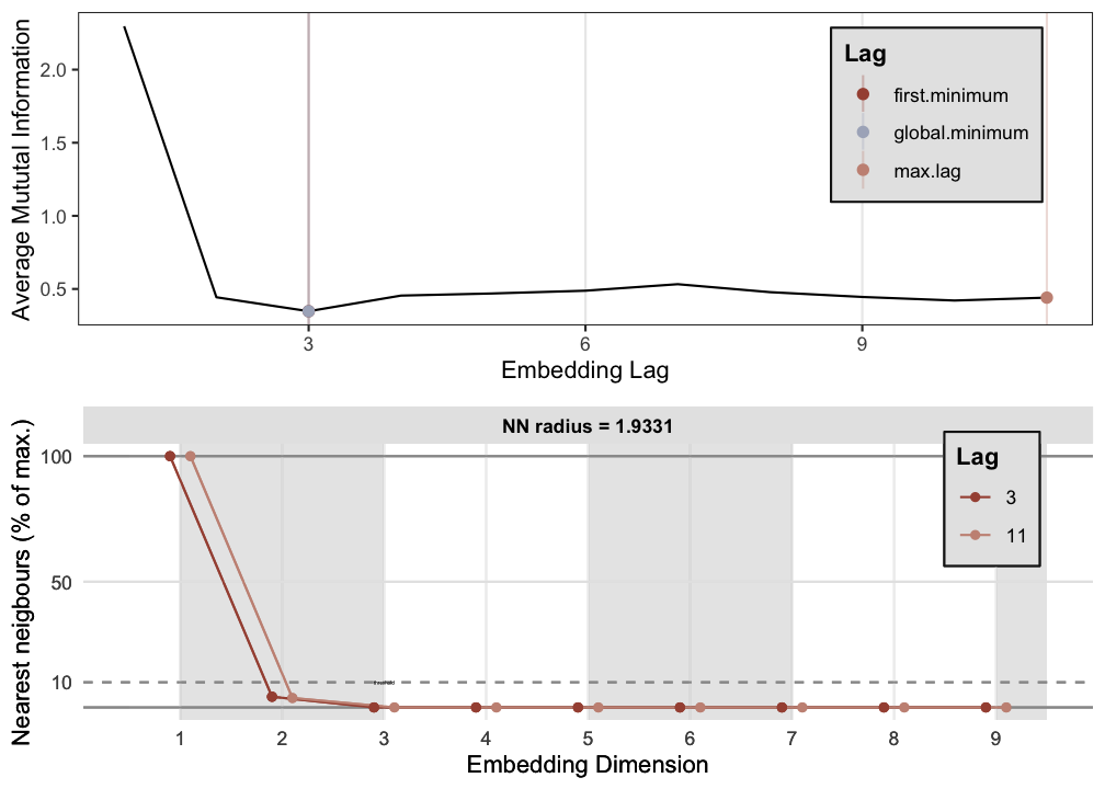

p2 <- est_parameters(y = out.cart$procrast)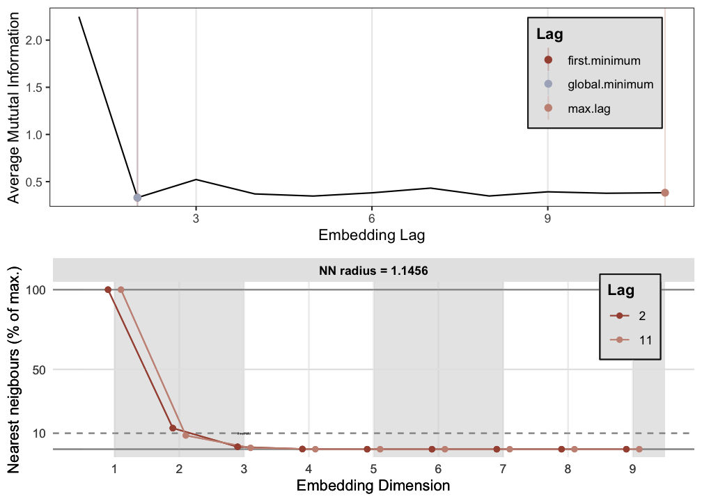

# By passing emRad = NA, a radius will be calculated based on 5% recurrence
RN1 <- casnet::rn(y1 = out.cart$restless, emDim = p1$optimDim, emLag = p1$optimLag, emRad = NA)
casnet::rn_plot(RN1)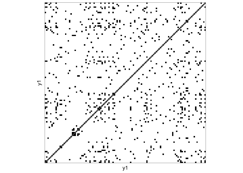

# Get RQA measures
rqa1 <- casnet::rp_measures(RN1, silent = FALSE)

> 
> ~~~o~~o~~casnet~~o~~o~~~
>  Global Measures
>   Global Max.points N.points     RR Singular Divergence Repetitiveness
> 1 Matrix      14161      887 0.0626      688     0.0084           1.65
> 
> 
>  Line-based Measures
>        Lines N.lines N.points Measure  Rate Mean Max.   ENT ENT_rel  CoV
> 1   Diagonal      41      199     DET 0.224 4.85  119 0.115  0.0240 3.76
> 2   Vertical      76      164   V LAM 0.185 2.16    3 0.436  0.0913 0.17
> 3 Horizontal      76      164   H LAM 0.185 2.16    3 0.436  0.0913 0.17
> 4  V+H Total     152      328 V+H LAM 0.185 2.16    3 0.436  0.0913 0.17
> 
> ~~~o~~o~~casnet~~o~~o~~~

# Create RN graph
g1  <- igraph::graph_from_adjacency_matrix(RN1, mode="undirected", diag = FALSE)
igraph::V(g1)$size <- igraph::degree(g1)
g1r <- casnet::make_spiral_graph(g1, 
                                 markEpochsBy = weeknum[1:vcount(g1)], 
                                 markTimeBy = TRUE)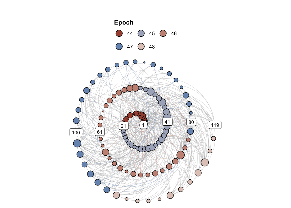

# Get RN measures
rn1 <- rn_measures(g1, silent = FALSE)

> 
> ~~~o~~o~~casnet~~o~~o~~~
> 
> Global Network Measures
> 
>   EdgeDensity MeanStrengthDensity GlobalClustering NetworkTransitivity
> 1  0.05469306                  NA        0.5443074           0.6294523
>   AveragePathLength GlobalEfficiency
> 1               Inf         7.585679
> 
> ~~~o~~o~~casnet~~o~~o~~~

# Should be the same
rqa1$RR==rn1$graph_measures$EdgeDensity

> [1] FALSE

TS 2

#----------------------
# Adjacency matrix TS_2
#----------------------
plot(ts(series$TS_2))

# Because these are generated signals, look for a drop in FNN below 1%.
p2 <- est_parameters(y = series$TS_2, nnThres = 1)

RN2 <- rn(y1 = series$TS_2, emDim = p2$optimDim, emLag = p2$optimLag, emRad = NA,  targetValue = 0.05)
rn_plot(RN2)

# Get RQA measures
rqa2 <- rp_measures(RN2, silent = FALSE)

# Create RN graph
g2 <- igraph::graph_from_adjacency_matrix(RN2, mode="undirected", diag = FALSE)
V(g2)$size <- degree(g2)
g2r <- make_spiral_graph(g2, arcs = arcs, epochColours = getColours(arcs), markTimeBy = TRUE)

# Get RN measures
rn2 <- rn_measures(g2, silent = FALSE)

# Should be the same
rqa2$RR==rn2$graph_measures$EdgeDensity

TS 3

#----------------------
# Adjacency matrix TS_3
#----------------------
plot(ts(series$TS_3))

# Because these are generated signals, look for a drop in FNN below 1%.
p3 <- est_parameters(y = series$TS_3, nnThres = 1)

RN3 <- rn(y1 = series$TS_3, emDim = p3$optimDim, emLag = p3$optimLag, emRad = NA, targetValue = 0.05)
rn_plot(RN3)

# Get RQA measures
rqa3 <- rp_measures(RN3, silent = FALSE)

# Create RN graph
g3 <- igraph::graph_from_adjacency_matrix(RN3, mode="undirected", diag = FALSE)
V(g3)$size <- degree(g3)
g3r <- make_spiral_graph(g3,arcs = arcs ,epochColours = getColours(arcs), markTimeBy = TRUE)

# Get RN measures
rn3 <- rn_measures(g3, silent = FALSE)

# Should be the same
rqa3$RR==rn3$graph_measures$EdgeDensity