6.3 Detrended Fluctuation Analysis (DFA)

The procedure for Detrended Fluctuation Analysis is similar to SDA, except that within each bin, the signal is first detrended, what remains is then considered the residual variance. The logic is the same, the way the average residual variance scales with the bin size should be an indication of the presence of power-laws. There are many different versions of DFA, one can choose to detrend polynomials of a higher order, or even detrend using the best fitting model, which is decided for each bin individually. See the manual pages of fd_dfa() for details.

dfaN1 <- fd_dfa(ColouredNoise$`-1`, doPlot = FALSE, returnPlot = TRUE, tsName = "Pink noise", noTitle = TRUE)

> 
> 
> (mf)dfa:  Sample rate was set to 1.
> 
> 
> ~~~o~~o~~casnet~~o~~o~~~
> 
>  Detrended FLuctuation Analysis 
> 
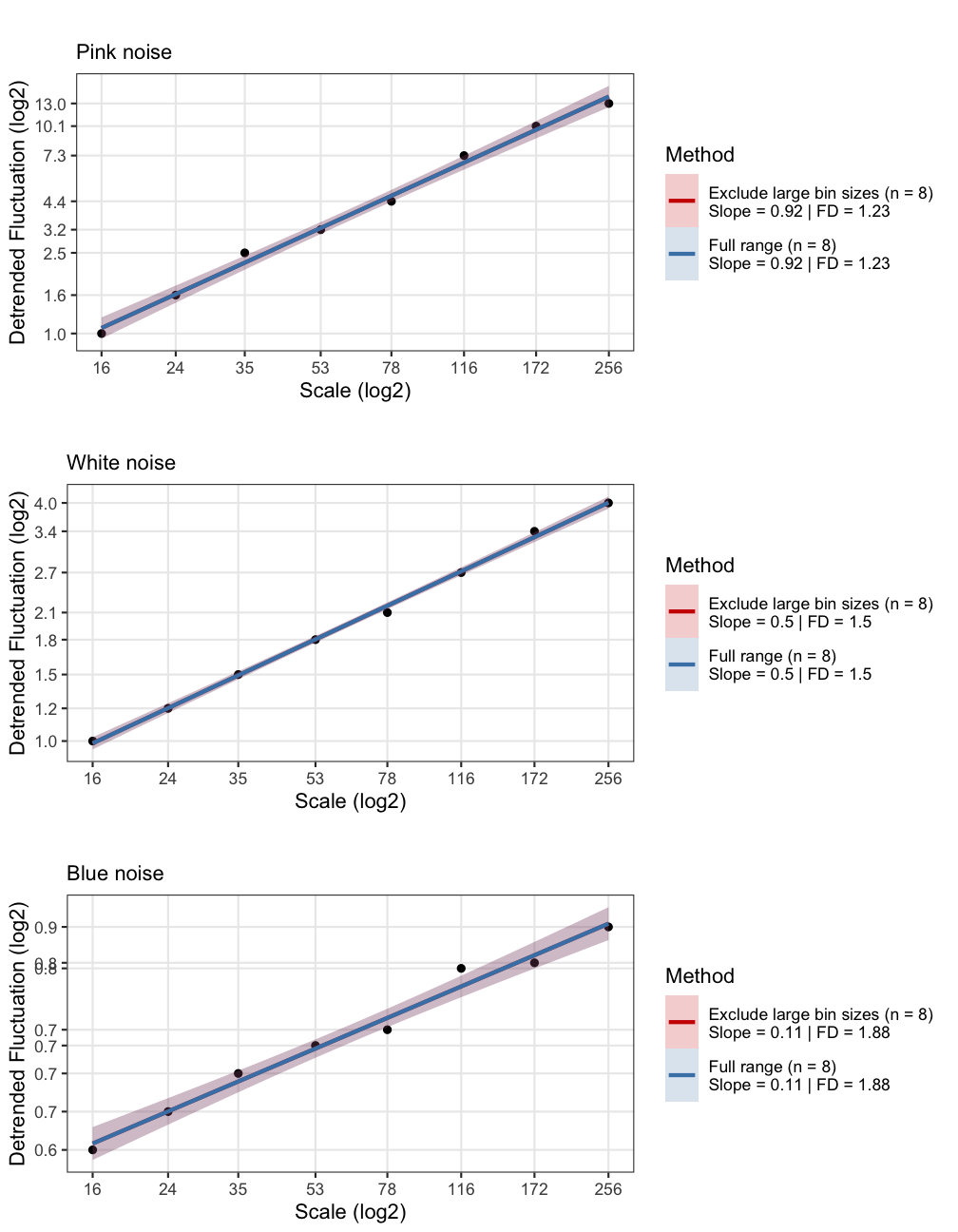
>  Full range (n = 8)
> Slope = 0.92 | FD = 1.23 
> 
>  Exclude large bin sizes (n = 8)
> Slope = 0.92 | FD = 1.23 
> 
>  Detrending: poly
> 
> ~~~o~~o~~casnet~~o~~o~~~

dfa0  <- fd_dfa(ColouredNoise$`0`, doPlot = FALSE, returnPlot = TRUE, tsName = "White noise", noTitle = TRUE)

> 
> 
> (mf)dfa:  Sample rate was set to 1.
> 
> 
> ~~~o~~o~~casnet~~o~~o~~~
> 
>  Detrended FLuctuation Analysis 
> 
>  Full range (n = 8)
> Slope = 0.5 | FD = 1.5 
> 
>  Exclude large bin sizes (n = 8)
> Slope = 0.5 | FD = 1.5 
> 
>  Detrending: poly
> 
> ~~~o~~o~~casnet~~o~~o~~~

dfaP1 <- fd_dfa(ColouredNoise$`1`, doPlot = FALSE, returnPlot = TRUE, tsName = "Blue noise", noTitle = TRUE)

> 
> 
> (mf)dfa:  Sample rate was set to 1.
> 
> 
> ~~~o~~o~~casnet~~o~~o~~~
> 
>  Detrended FLuctuation Analysis 
> 
>  Full range (n = 8)
> Slope = 0.11 | FD = 1.88 
> 
>  Exclude large bin sizes (n = 8)
> Slope = 0.11 | FD = 1.88 
> 
>  Detrending: poly
> 
> ~~~o~~o~~casnet~~o~~o~~~

cowplot::plot_grid(dfaN1$plot,dfa0$plot,dfaP1$plot,ncol = 1)