3.2 No! … It’s a time series!
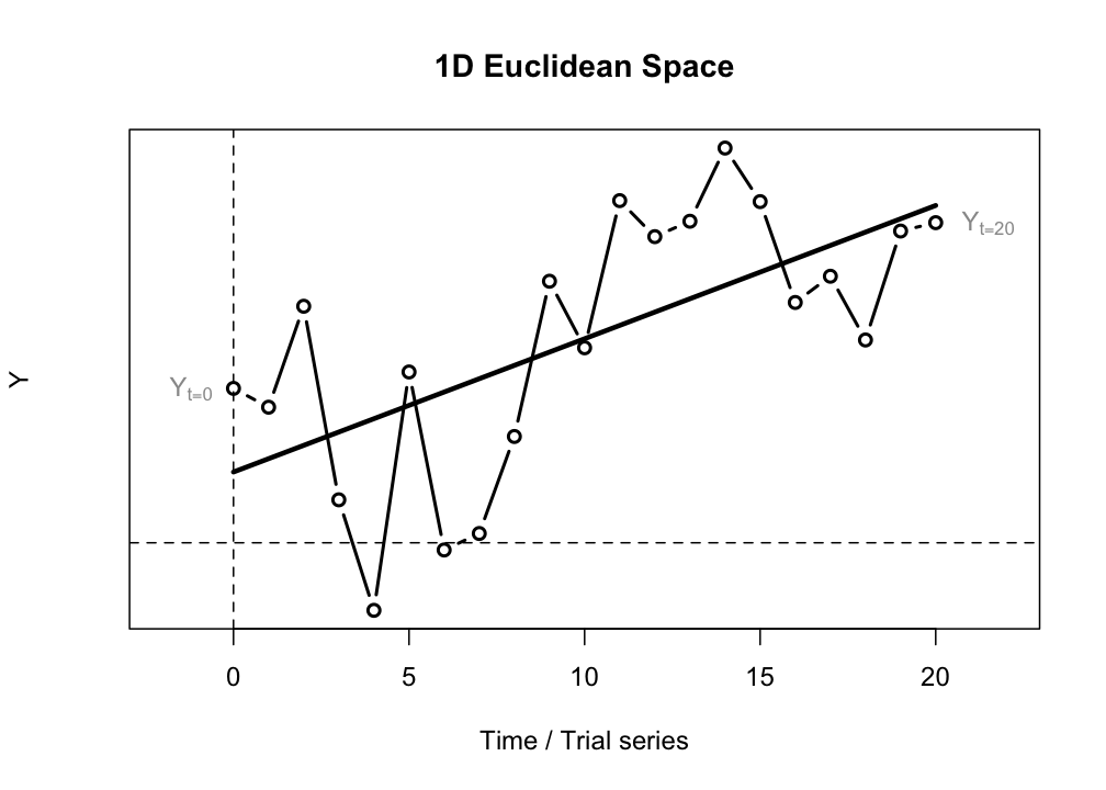
The important difference between a regular 2-dimensional Euclidean plane and the space in which we model change processes is that the \(X\)-axis represents the physical dimension time. In the case of the Linear Map we have a 1D space with one ‘spatial’ dimension \(Y\) and a time dimension \(t\) (or \(i\)). This is called a time series if \(Y\) is sampled as a continuous process, or a trial series if the time between subsequent observations is not relevant, just the fact that there was a temporal order (for example, a series of response latencies to trials in a psychological experiment in the order in which they were presented to the subject).
Time behaves different from a spatial dimension in that it is directional (time cannot be reversed), it cannot take on negative values, and, unless one is dealing with a truly random process, there will be a temporal correlation across one or more values of \(Y\) separated by an amount of time. In the linear difference equation this occurs because each value one step in the future is calculated based on the current value. If the values of \(Y\) represent an observable of a dynamical system, the system can be said to have a history, or a memory.
Ergodic systems do not have a history or a memory that extends across more than a sufficiently small time scale (e.g. auto-correlations at lags of ±1-5 can be expected, but there should be no systematic relationships that span several decades). Assuming such independence exists is very convenient, because one can calculate the expected value of a system observable (given infinite time), by making use of of the laws of probabilities of random events (or random fields). This means: The average of an observable of an Ergodic system measured across infinite time (its entire history, the time-average), will be the be the same value as the average of this observable measured at one instance in time, but in an infinite amount of systems of the same kind (the population, the spatial average) [^dice].
The simple linear growth difference equation will always have a form of perfect memory across the smallest time scale (i.e., the increment of 1, from \(t\) to \(t+1\)). This ‘memory’ just concerns a correlation of 1 between values at adjacent time points (a short range temporal correlation, SRC), because the change from \(Y_t\) to \(Y_{t+1}\) is exactly equal to \(a * Y_t\) at each iteration step. This is the meaning of deterministic, not that each value of \(Y\) is the same, but that the value of \(Y\) now can be perfectly explained form the value of \(Y\), one moment in the past.
Summarising, the most profound difference is not the fact that the equation of linear change is a deterministic model and the GLM is a probabilistic model with parameters fitted from data, this is something we can (and will) do for \(a\) as well. The profound difference between the models is the role given to the passage of time:
- The linear difference equation represents changes in \(Y\) as a function of the physical dimension time and \(Y\) itself.
- The GLM represents changes in \(Y\) as a function of a linear predictor composed of additive components that can be regarded as independent sources of variation that sum up to the observed values of \(Y\).
Figure 3.1 shows the main differences between the GLM and Differential/Difference equation models.
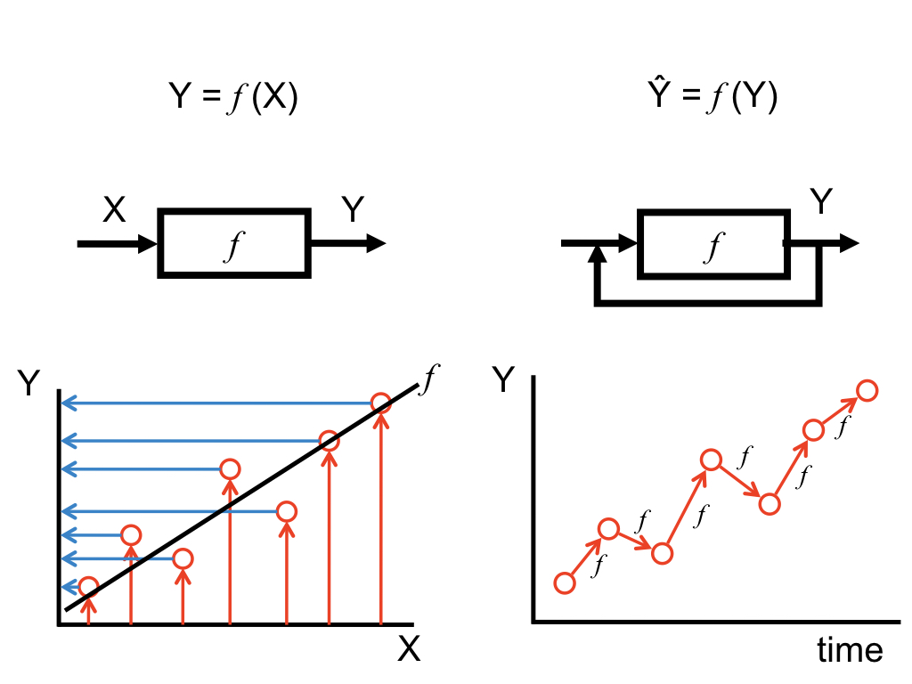
Figure 3.1: General Linear Model versus Differential/Difference equations