C.1 Univariate imputation

In addition to useful summary and visualisation tools, package imputeTS contains a number of imputation methods that are commonly used. If you have installed the package, run vignette("imputeTS-Time-Series-Missing-Value-Imputation-in-R", package = "imputeTS") from the console ans learn about all the options.

Linear interpolation

One of the most straightforward inputation methods is linear interpolation. This is a relatively sensible method if there is just one time point missing. However, when several values are missing in a row, the linear interpolation might be unrealistic. Other methods that will give less plausible results for imputation of multiple missing values in a row are last observation carried forward and next observation carried backward, also available in imputeTS as na_locf(type = "locf"), and na_locf(type = "nocb") respectively.

We’ll generate a data set with linear interpolation (also available are spline and stine interpolation), to compare to the more advanced multiple imputation methods discussed below.

out.linear <- t(laply(1:NCOL(df_vars), function(c){
  y  <- as.numeric(as.numeric_discrete(x = df_vars[,c], keepNA = TRUE))
  idNA <- is.na(y)
  yy <- cbind(imputeTS::na_interpolation(y,option = "linear"))
  if(all(is.wholenumber(y[!idNA]))){
    return(round(yy))
  } else {
      return(yy)
    }
  }))
colnames(out.linear) <- colnames(df_vars)

Note that we need to round the imputed values to get discrete values if the original variable was discrete.

Kalman filter

Imputation by using the Kalman filter is a powerful method for imputing data. However, when dealing with discrete data, one has to take some additional steps in order to get meaningful results.

For example, with uniform discrete numbers and/or scales that are bounded (eg. visual analog scale from 0-100), the Kalman method will not correctly impute the data and might go outsdide the bounds of the scale.

# Use casnet::as.numeric_discrete() to turn a factor or charcter vector into a named numeric vector.
ca <- as.numeric_discrete(df_vars$cat_ordered, keepNA = TRUE)
imputations <- imputeTS::na_kalman(ca, model = "auto.arima")
imputeTS::ggplot_na_imputations(x_with_na = ca, x_with_truth = as.numeric_discrete(cat_ordered), x_with_imputations = imputations)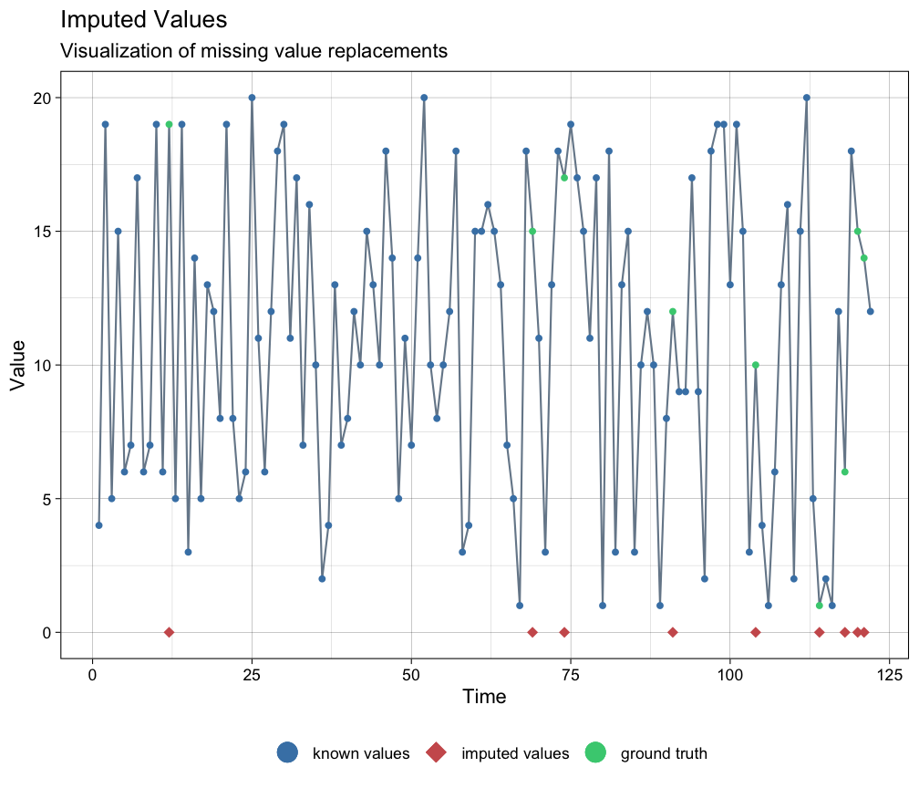

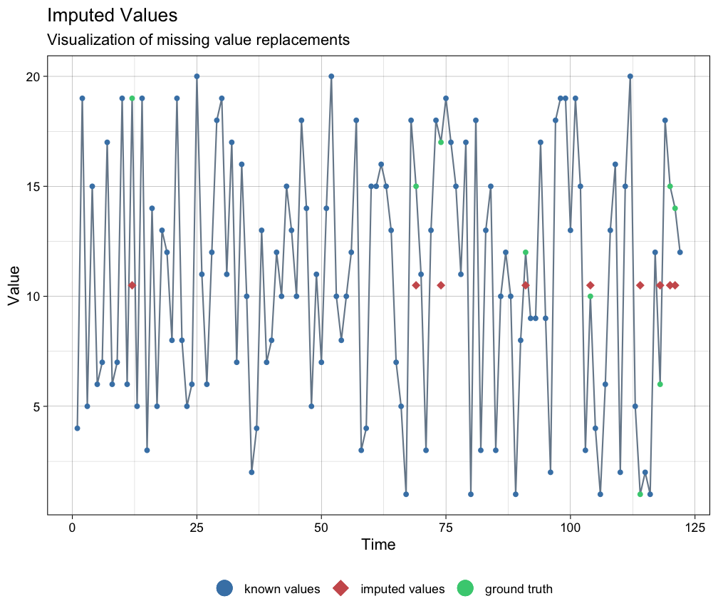
There is a way to adjust the imputation procedure by transforming the data (thanks to Steffen Moritz, author of imputeTS, for suggesting this method). The ordered categorical series was created with bounds 1 and 20.

# Bounds 
lo <- 1
hi <- 20
# Transform data, take care of dividsion by 0
ca_t <- log(((ca-lo)+.Machine$double.eps)/((hi-ca)+.Machine$double.eps))
imputations <- imputeTS::na_kalman(ca_t, model = "auto.arima")
# Plot the result
# Back-transform the imputed forecasts 
imputationsBack <- (hi-lo)*exp(imputations)/(1+exp(imputations)) + lo

imputeTS::ggplot_na_imputations(x_with_na = ca, x_with_truth = as.numeric_discrete(cat_ordered), x_with_imputations = imputationsBack)