6.1 Power Spectral Density (PSD) slope

Power Spectral Density slope analysis first transforms the time series into the frequency domain by performing the Fourier transform. This breaks down the signal into sine and cosine waves of a particular amplitude that together “add-up” to represent the original signal. If there is a systematic relationship between the frequencies in the signal and the power of those frequencies (power = amplitude^2), this will reveal itself in log-log coordinates as a linear relationship. The slope of the best fitting line is taken as an estimate of the scaling exponent and can be converted to an estimate of the fractal dimension.

Package casnet contains a dataset called ColouredNoise, the column names represent the scaling exponent of the time series simulated with noise_powerlaw().

casnet::plotTS_multi(ColouredNoise)

Data preparation usually involves the steps required for conducting the Fourier analysis. This includes centring on the mean (or standardising) and detrending the time series (the Fourier transform is a linear technique which assumes stationarity).

Calling fd_psd() will produce a summary output in the console. For all functions of the fd_ family, two scaling exponents will be estimated, one based on the entire range of data points that represent a potential powerlaw, and one based on a restricted range. In the case of the spectral slope, it is custom to fit only over the scaling region in the lower frequencies (for negative scaling exponents) or higher frequencies (for positive scaling exponents). See the fitMethod argument in the manual for an explanation of the options for selecting a range of frequencies.

psdN1 <- fd_psd(ColouredNoise$`-1`, returnPlot = TRUE, tsName = "Pink noise", noTitle = TRUE, doPlot = FALSE, )

> 
> 
> (mf)dfa:  Sample rate was set to 1.
> 
> 
> ~~~o~~o~~casnet~~o~~o~~~
> 
>  Power Spectral Density Slope 
> 
>  All frequencies (n = 512)
> Slope = -1.06 | FD = 1.19 
> 
>  Hurvich-Deo (n = 81)
> Slope = -1.04 | FD = 1.19
> 
> ~~~o~~o~~casnet~~o~~o~~~

psd0 <- fd_psd(ColouredNoise$`0`, returnPlot = TRUE, tsName = "White noise", noTitle = TRUE, doPlot = FALSE)

> 
> 
> (mf)dfa:  Sample rate was set to 1.
> 
> 
> ~~~o~~o~~casnet~~o~~o~~~
> 
>  Power Spectral Density Slope 
> 
>  All frequencies (n = 512)
> Slope = -0.12 | FD = 1.45 
> 
>  Hurvich-Deo (n = 34)
> Slope = -0.35 | FD = 1.37
> 
> ~~~o~~o~~casnet~~o~~o~~~

psdP1 <- fd_psd(ColouredNoise$`1`, returnPlot = TRUE, tsName = "Blue noise", noTitle = TRUE, doPlot = FALSE)

> 
> 
> (mf)dfa:  Sample rate was set to 1.
> 
> 
> ~~~o~~o~~casnet~~o~~o~~~
> 
>  Power Spectral Density Slope 
> 
>  All frequencies (n = 512)
> Slope = 1.02 | FD = 1.8 
> 
>  Hurvich-Deo (n = 85)
> Slope = 0.82 | FD = 1.76
> 
> ~~~o~~o~~casnet~~o~~o~~~

cowplot::plot_grid(psdN1$plot,psd0$plot,psdP1$plot,ncol = 1)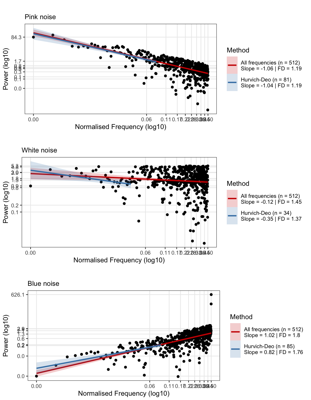

The sample time series were generated using the inverse Fourier transform. Therefore, the fd_psd() estimates are expected to yield most accurate estimates the scaling exponent. Let’s see how other approaches do.