B.3 The return plot

To create a return plot the values of \(Y\) have to be shifted by a certain lag. The functions lead() and lag() in package::dplyr are excellent for this purpose (note that dplyr::lag() behaves different from stats::lag()).

# Function lag() and lead()
library(dplyr)
library(casnet)

# Get exponential growth
YY <- growth_ac(N=1000,r=1.5,type = "driving")
Y1 <- as.numeric(YY/max(YY))
# Get logistic growth in the chaotic regime
Y2 <- as.numeric(growth_ac(N=1000,r=4,type = "logistic"))
# Use the `lag` function from package `dplyr`
op <- par(mfrow = c(1,2), pty = "s")
plot.ts(dplyr::lag(Y1), Y1, xy.labels = FALSE, pch = 16, xlim = c(0,1), ylim = c(0,1), xlab = "Y(t)", ylab = "Y(t+1)",
     main = "exponential / max")
plot.ts(dplyr::lag(Y2), Y2, xy.labels = FALSE, pch = 16, xlim = c(0,1), ylim = c(0,1), xlab = "Y(t)", ylab = "Y(t+1)",
     main = "logistic / max")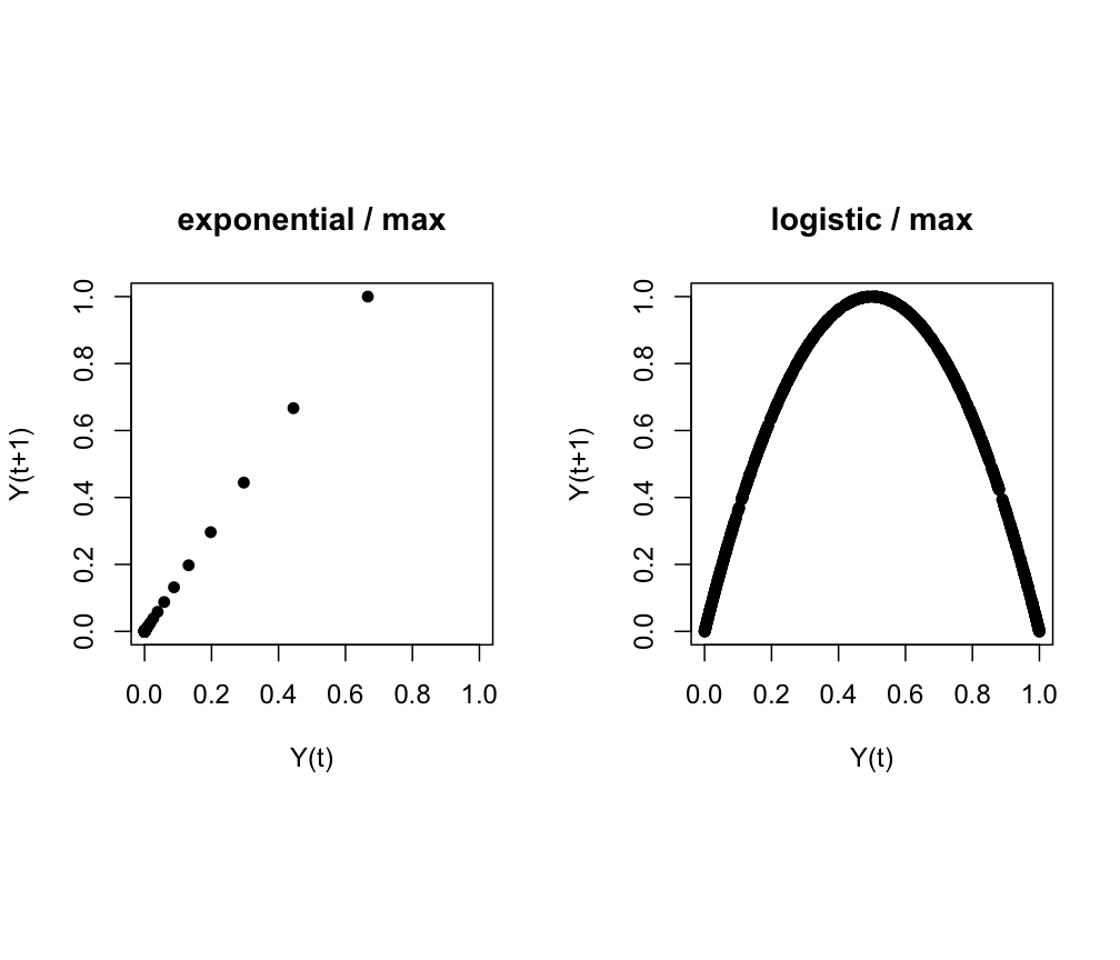

par(op)

Use l_ply() from package::plyr to create return plots with different lags. The l_ before ply means the function will take a list as input to a function, but it will not expect any data to be returned, for example in the case of a function that is used to plot something.

# Explore different lags
op <- par(mfrow = c(1,2), pty = "s")
plyr::l_ply(1:4, function(l) plot.ts(dplyr::lag(Y2, n = l), Y2, xy.labels = FALSE, pch = 16, xlim = c(0,1), ylim = c(0,1), xlab = "Y(t)", ylab = paste0("Y(t+",l,")"), cex = .8))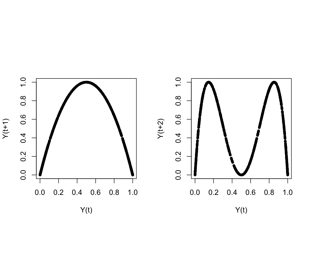

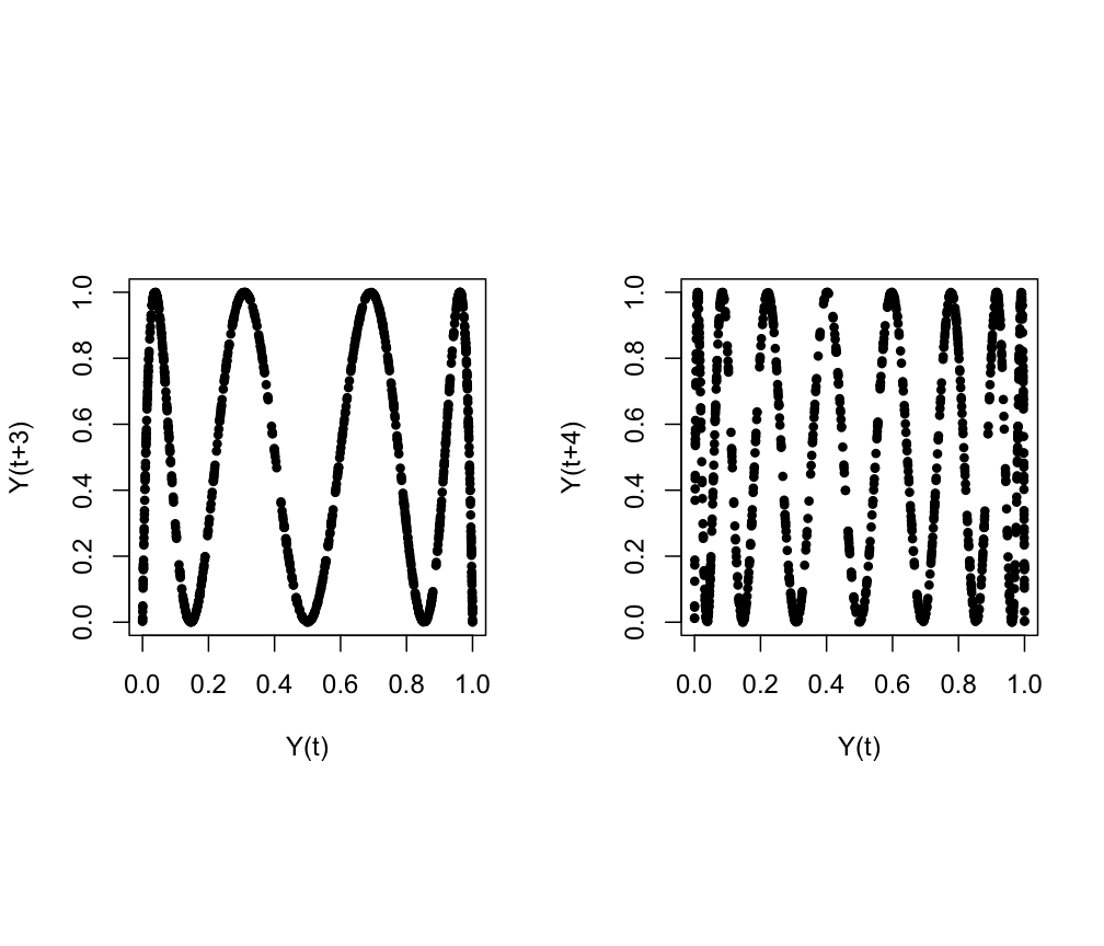
par(op)